A quick review of Algorithms and data structures
Notes are taken from the Pluralsight course Algorithms and data structures by the crack Robert Horvick
Disclaimer: Most of the images and code are taken from the course. If I am breaking any Copyright rules, please let me know.
Table of Contents
- Storing and Accessing Data
- Asymptotic Analysis of Algorithms
- Linked Lists
- Stacks and Queues
- Binary Search Trees
- Hash Tables
- Sorting and Searching Array Data Structures
- String Searching Algorithms
- Balanced Binary Trees
- Sets and Set Algorithms
- B-Trees
- Heaps and Priority Queues
- Collection Concurrency
- Resources
Other usefull links
Binary Search Algorithm Explained
How Big O Notation Works – Explained with Cake
Storing and Accessing data
Storing and accessing data is a fundamental part of any programming language. This topic will help us cover creating, adding, and updating array data, and also we will scope Enumerating array data.
One of the most important topics is when we work with an array is to measure the algorithmic complexity of the operations. That can be accomplished using asymptotic analysis or by using the Big O notation.
So, we will start defining why arrays?
- An array can continue multiple instances of a type.
- Can be numeric indexing.
- You can access individual items.
- Static of dynamic size.
- Fixed-size once is created.
Creating an array
1 |
|
Asymptotic analysis of Algorithms
An algorithm consumes Resources like:
- Operations: The number of times we need to perform some operations
- Memory: How much memory is consumed by the algorithms.
- Others: Network transfer, compression ratios, disk usage.
1 |
|
The algorithm will start comparing after was found the value ‘G’. Each operation has a cost of 1 associated with it. In this example, the algorithm will perform 7 operations and that will be the cost of the algorithm. The length of the array will be call N.
Big O notation
That is the way to measure the complexity of the algorithms. The Big O notation is a way to represent the upper limit of the algorithm cost. And is associated with the big O(n) and N as the size of the input.
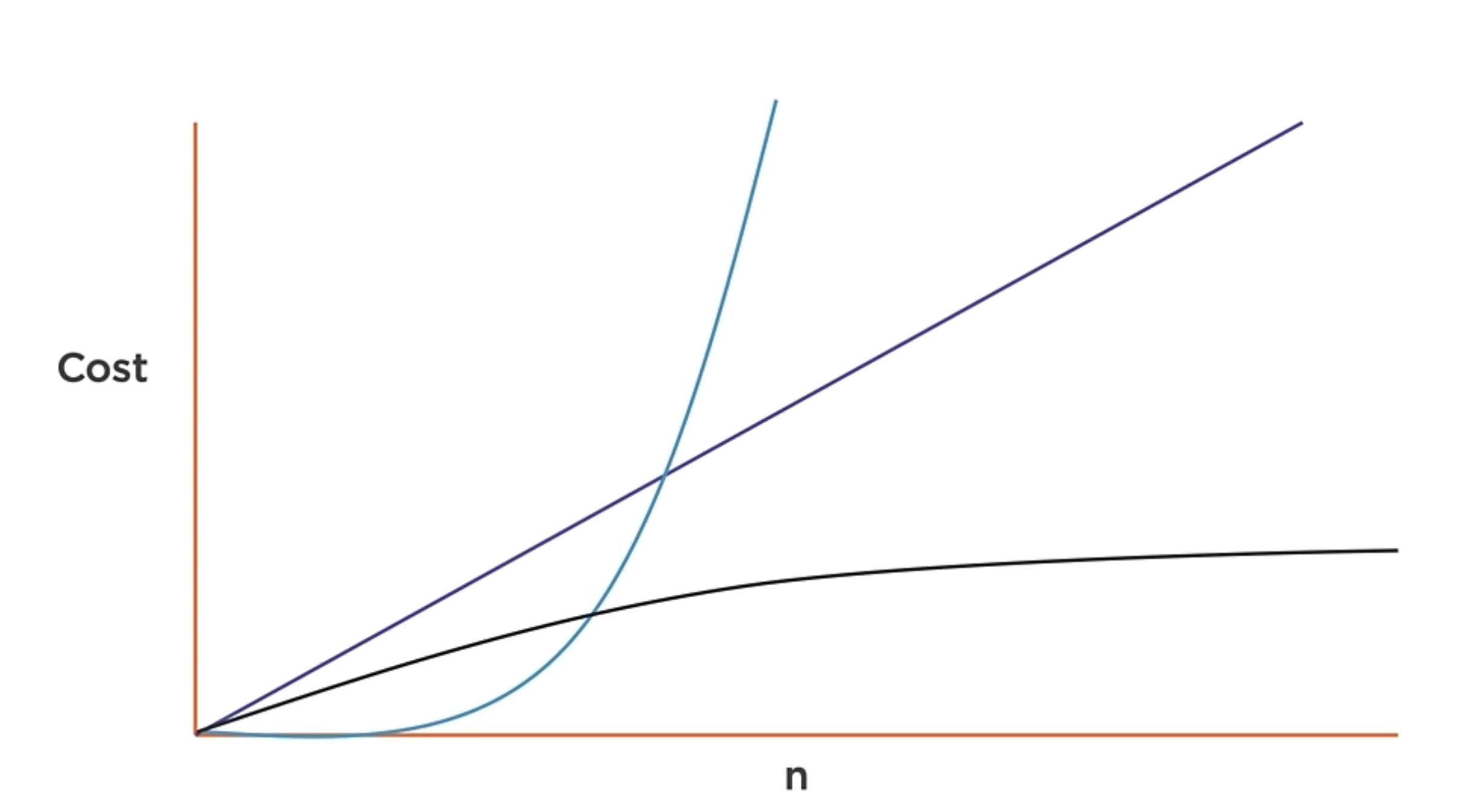
O(n+1) is O(n)
O(2n) is O(n)
These two expressions are the same because the algorithm will perform the lineal curve.
Some algorithms have a fixed cost regardless of the input size. But don’t confuse fix size with fast, because the input can be very large. The point is that the amount of work that is done is not dependent on the input size.
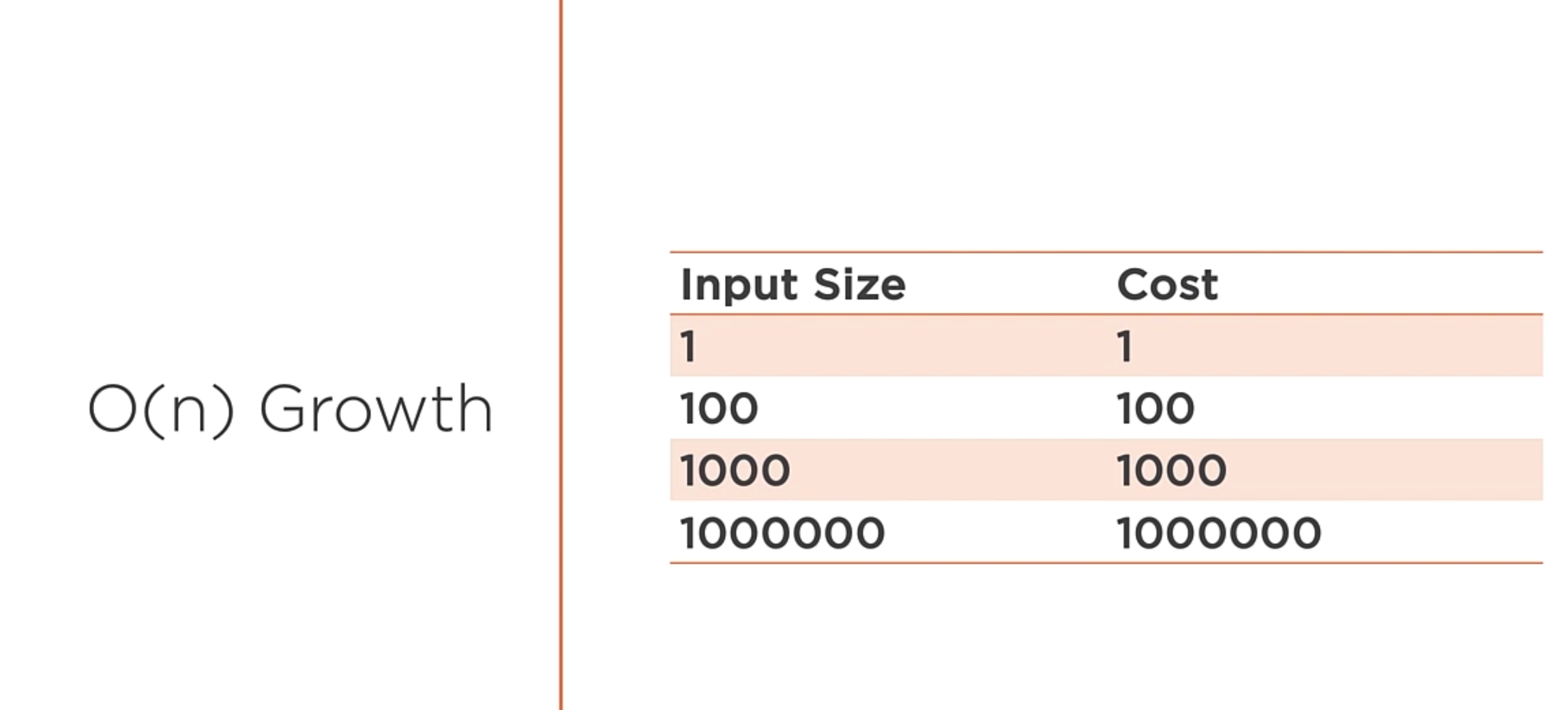
O(n) is a function whose cost scales linearly with the size of the input.
1 |
|
O(n)
Iterating over a collection of data once often indicates an O(n) algorithm. If the n changes, the algorithm will still be O(n). You can identify this as a linear algorithm because you can see a single loop over the collection of data.
O(log n)
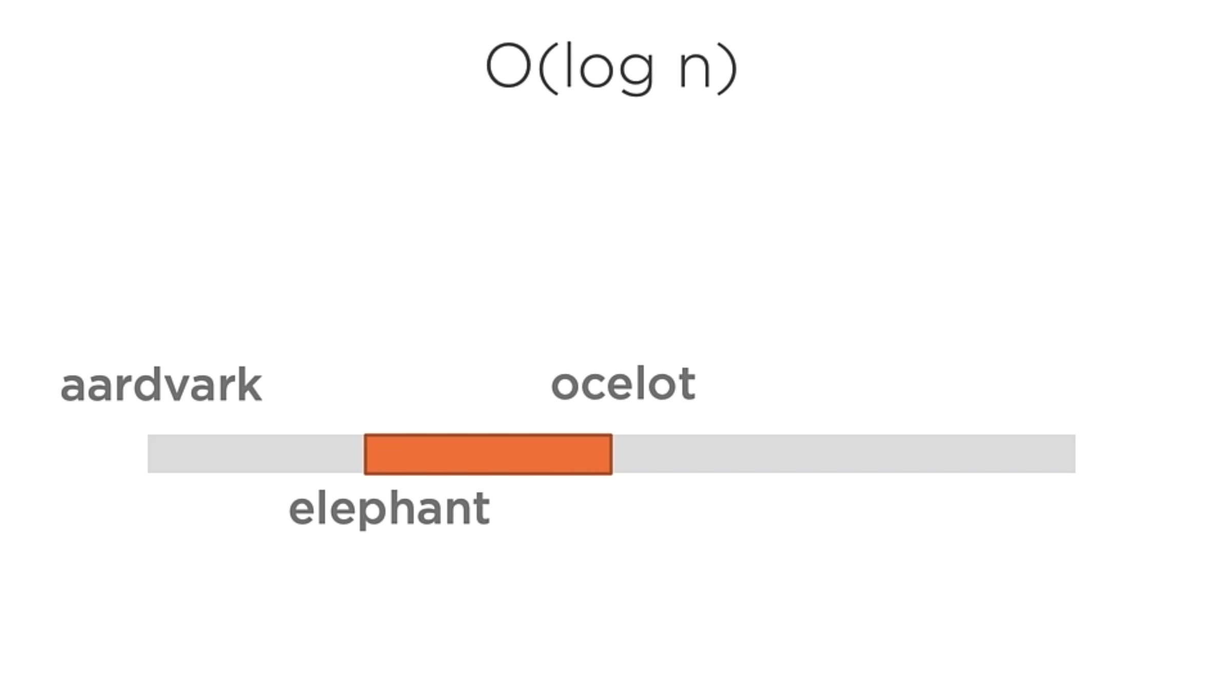
A function whose cost scales logarithmically with the input size. Works dividing large problems into smaller and smaller chunks. This is the case for binary search.
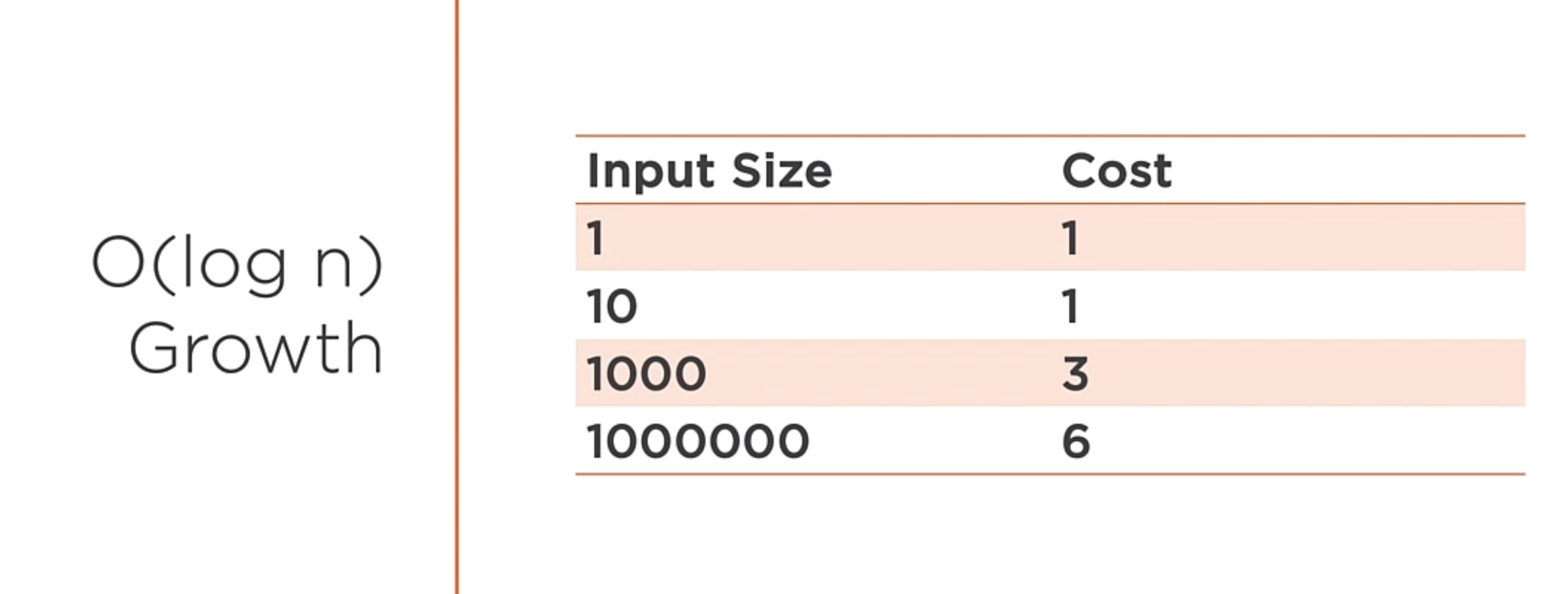
It is different from the O(n) because as the size of the input grows, the cost of the algorithm does not increase in the same way.
O(n^2)
A function that exhibits quadratic growth relative to the input size. A doubly-nested loop is an indication that you might have an O(n^2) algorithm. This is the case for bubble sort.
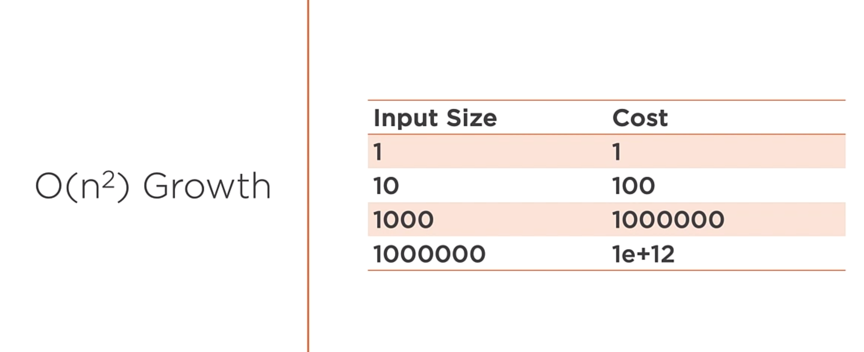
1 | void quad(char[] input, int count){ |
O(nm)
A function which has two inputs that contribute to the growth. This is the case for matrix multiplication.
1 |
|
A nested loop that iterates over two distinct collections of data might indicate an O(nm) algorithm. The problem with this type of algorithm is that you need to understand your domain because both inputs are O(n) algorithms.
Big O summary
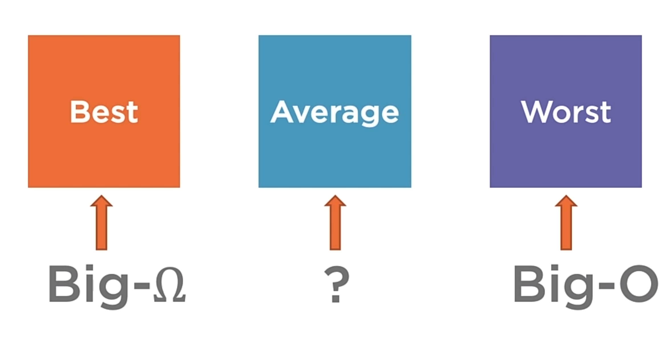
This is a way to measure the worst-case complexity of the algorithms.
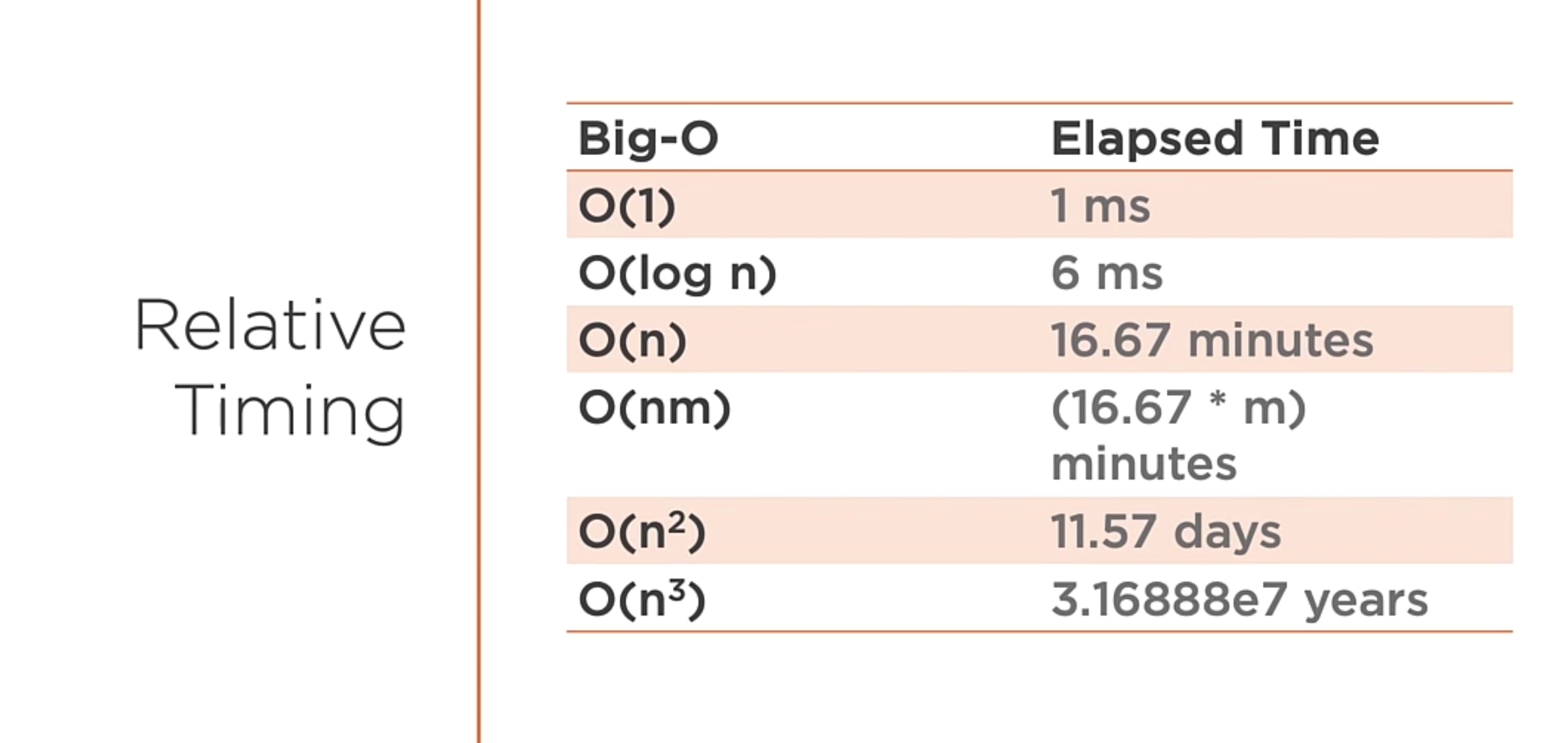
As you can see in the image above, there is a differente ways to measure the relative time between the algorithms.
Linked Lists
A container where data is stored in nodes consisting of a single data item and a reference to the next node.
The concept of a linked list is similar to a chain. When you start at the first link and follow the chain to the last link. You can’t jump from the first to the second and iterate through the list.
Each link of the chain has a node. Each node has a single value and a reference to the next node.
Example of a Node Class pointing to the next node
1 |
|
Singly Linked List
A linked list that provides forward iteration from the start to the end of the list.
Example of a LinkedListNode Class that points to the next node when are created
1 | class LinkedListNode<TNode>{ |
The singly linked list node is a generic class containing the data and the reference to the next node
Doubly Linked List
A linked list that provides forward iteration from the start to the end of the list, and reverse iteration, from the end to start.
Example of a Node Class that allows point to the next node and previous
1 |
|
Linked List summary
A linked list is a collection of nodes chains together. Each node has a value and a reference to the next node. We can perform operations on the list like:
- Adding and removing nodes
- Adding nodes ordered by value
- Enumeration
- Searching
Stacks and Queues
- Stacks: The last-in, First-out data structure.
- Queues: The First-in, First-out data structure.
- Deque: Double-end queue.
Stack
Last-in, First-out (LIFO) data structure. Follow the rule the last item added is the first item removed.
When you remove (a.k.a Pop) an item from a stack, you remove the tail that is the last item added.
Queue
A first-in, first-out (FIFO) data structure. “Queuing” into a line, so the first item added is the first item removed. So, the First item is the “head” of the list, and the last is the “tail” in the list.
So, when you remove an item from a queue, you remove the head of the list. If you add a new item to the queue, the new item is added to the tail of the list.
Doubly Ended Queue
A queue-like container which is both First-in, First-out and Last-in, Last-out.
Start with an empty queue
1 | [ , , , , ] |
Add “3” to the head of the queue. Right now, the queue is empty, so it doesn’t matter what the head and tail are. The queue is now:
1 | [ , , , , 3 ] |
Add “2” to the tail. The queue is now:
1 | [ , , , 2 , 3 ] |
Add “4” to the head. 4 is now the head of the queue, moving the number 3 of his position. The queue is now:
1 | [ , , 2 , 3 , 4 ] |
Add “1” to the tail. That makes the number 1 to the tail and leaves the Head unchanged. The queue is now:
1 | [ , 1 , 2 , 3 , 5 ] |
Finally, add “5” to the head. That makes the number 5 to the head and leaves the tail unchanged. The queue is now:
1 | [ 1 , 2 , 3 , 4 , 5 ] |
Remove “5” from the head. This is just a dequeue operation, when we remove the item at the start of the queue. The queue is now:
1 | [ , 1 , 2 , 3 , 4 ] |
Now remove the “1” from the tail of the queue. This behaviour isn’t like dequeue because we aren’t removing the head, but it’s also not quite like the stack because the value 1 wasn’t necessarily the last item added to the container. The queue is now:
1 | [ , , 2 , 3 , 4 ] |
Now remove 2 from the tail of the container. Leaving 3 and 4 in the doubly ended queue. The queue is now:
1 | [ , , , 3 , 4 ] |
Now remove 4 from the head of the container. Leaving only a single value of 3. The queue is now:
1 | [ , , , , 3 ] |
With only a single value left, we can remove it from the head or the tail leaving the same effect, leaving the container empty.
Implementation.
Let’s put this all together.
1 | public class Deque<T> : IEnumerable<T> |
In the code above, we create a new class called Deque. This class uses a DoublyLinkedList to store the data. That allows us to add and remove items from the head and tail of the list.
Now that we understand how DoublyLinked Deque works, let’s implement it with a Queue class and Stack class.
1 |
|
In the code above, we create a new class called Queue. This class uses a DoublyLinkedList to store the data. The behavior of Enqueue and Dequeue is enqueued tail and dequeue head.
The reason this works is because when we add an item to the tail of the list, we progressively pushing the older and older item to the head. So When you add your fist item to the tail, it’s both the head and the tail. When you add your second item to the tail, the original item is still the head, but the new item is the tail.
So, the basic idea with the Queue is you remove items from the head and add items to the tail.
Also, the class has the Peek method defers to PeekHead on the Deque.
1 | public class Stack<T> |
In the code above, we create a new class called Stack. This class is pretty similar to the Queue class. The difference is instead of adding items to the head and taking them from the tail, we add items to the head and take them from the head.
So, the basic idea with the Stack is the last item that we add to the head is the first item that we take from the head.
Binary Search Trees
A data structure where nodes have a 1:N parent-child relationship.
Parts of the Tree
The trees begins at the root part. Then, the tree expands with branches. The branches are internal to the tree and expand outward. And eventually, we get to the leaves. The leaves are the end of the branches.
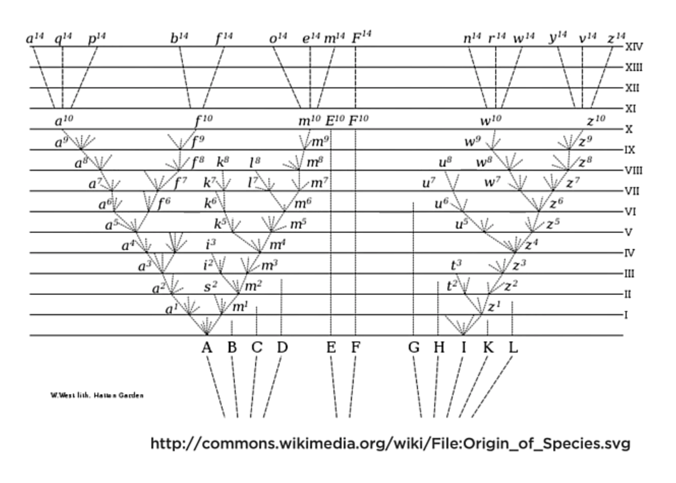
Categorization of the species as a tree representation
Properties of trees
Binary Trees
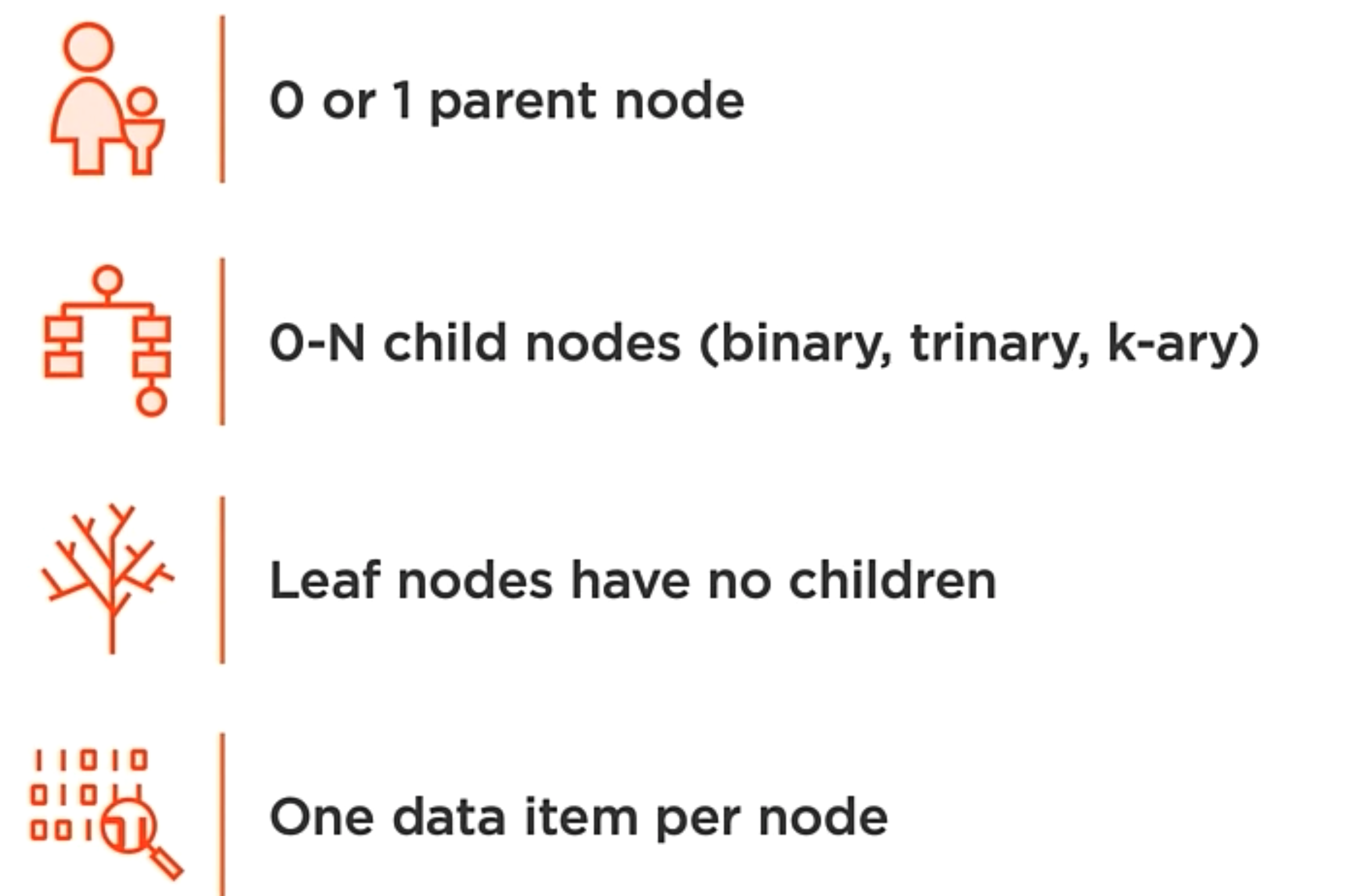
- Starts with a root node.
- Nodes has parents and children relationships.
- The connection between nodes is made with Edges.
- Nodes that have no children are referred to as Leaf nodes.
- Internal nodes are the nodes that are neither the root nor the leaf node.
- The degree of the Tree, is max number of children each node can have.
- The height of the node is the maximun number of edges between that node and the leaf node.
- The level counts the edges to root node.
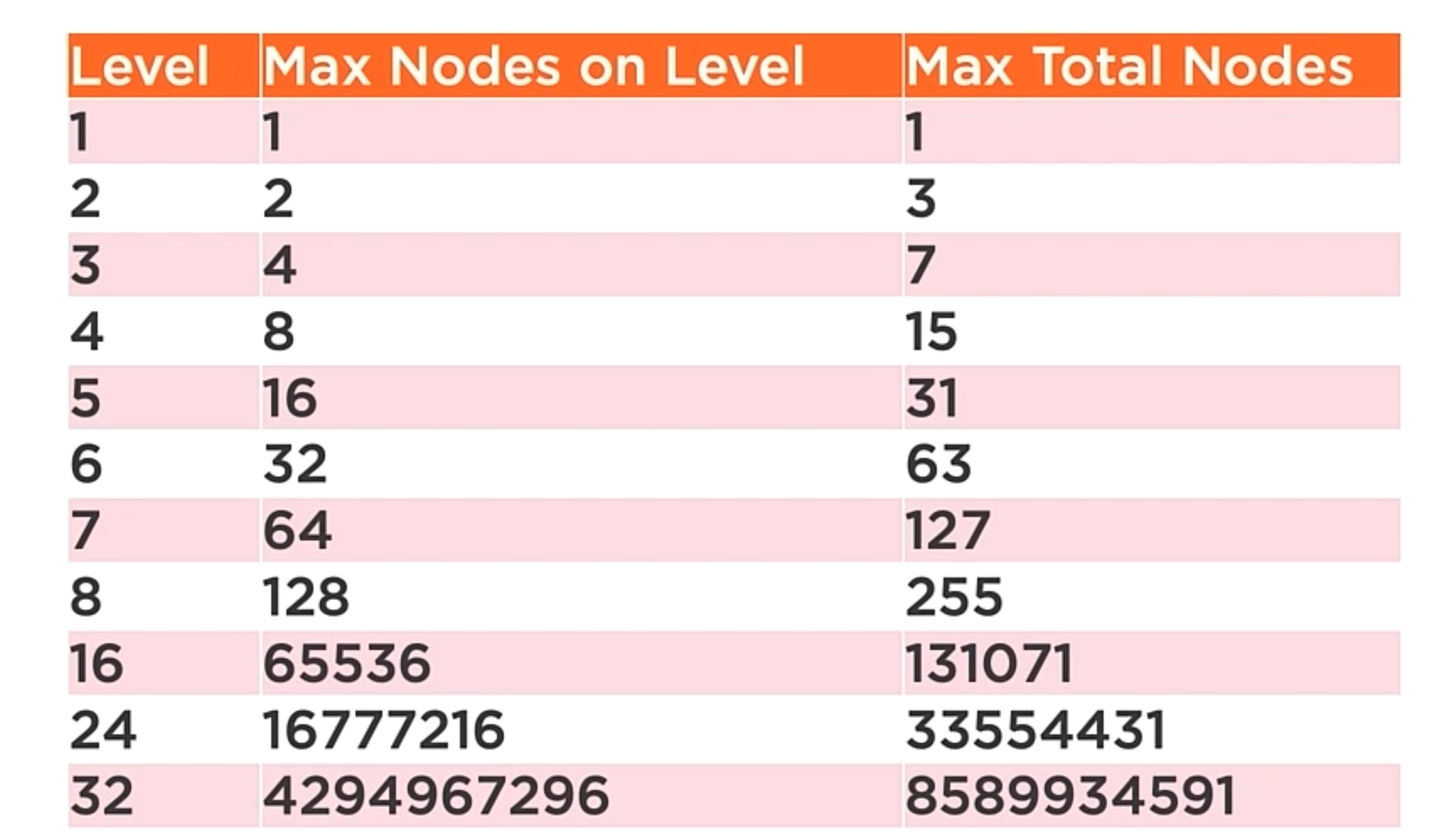
Binary tree nodes per level
Basic Operations
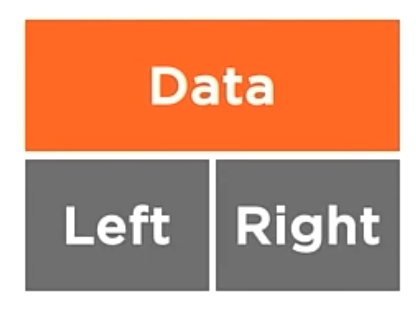
1 | class BSTNode<T>{ |
In the code above, we create a new class called BSTNode. This class has two properties, Left and Right. These properties are the nodes that are the left and right children of the node. The class also has a property called Data. This property is the data that the node holds.
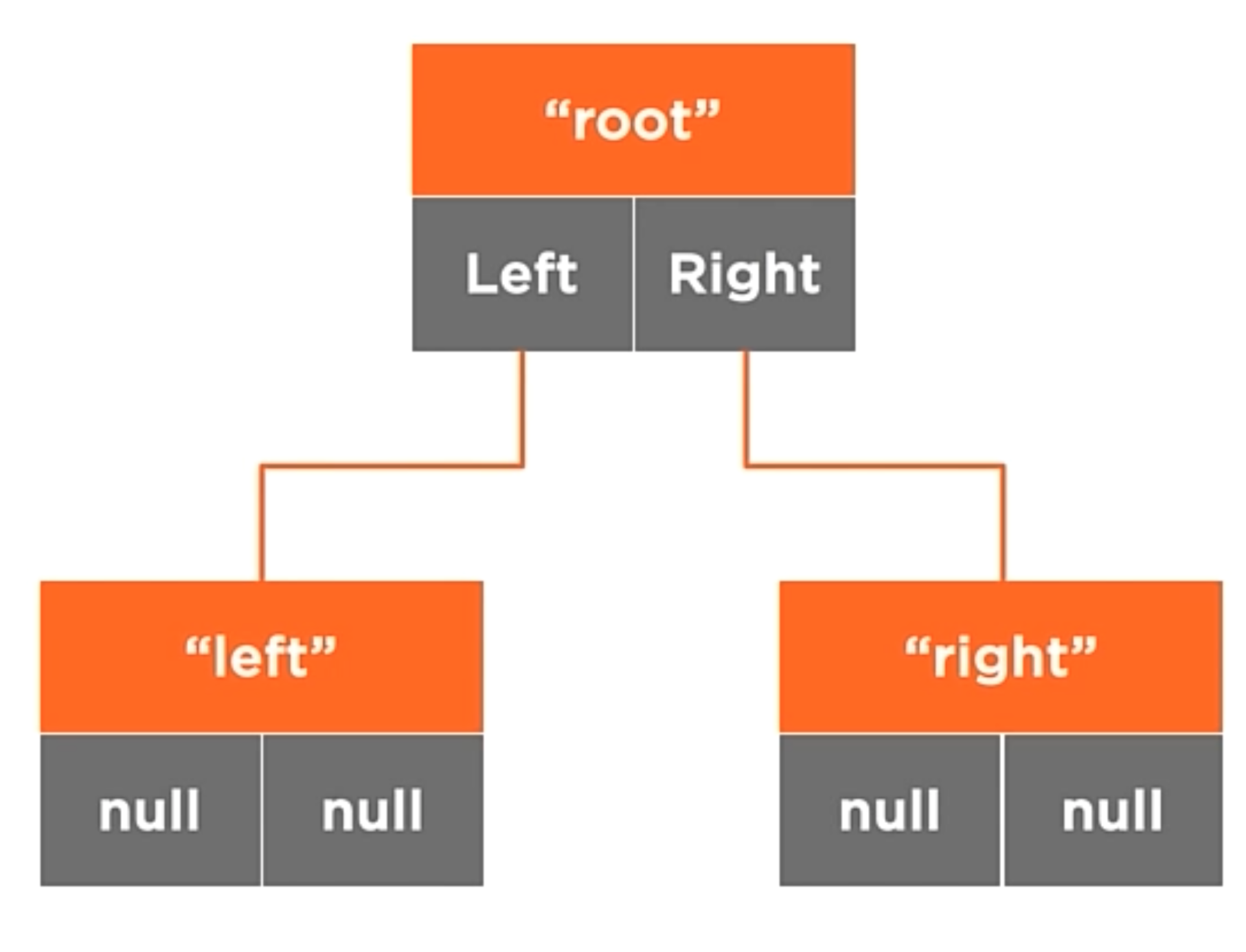
1 | BSTNode<string> root = new BSTNode<string>("root"); |
In the code above, we create a new node called root. This node has two children, left and right. The data is set to “root”.
Binary search Tree
A binary tree where nodes with the lower values are places to the left of the root, and nodes with equal or greater values are places to the right.
The tree has types of rules that are related to the domain. These rules are constraints on the tree and it seems to limit, that actually allow the tree to function as a more useful data structure.
So, when values are added to the tree, smaller values go to the left. For example:
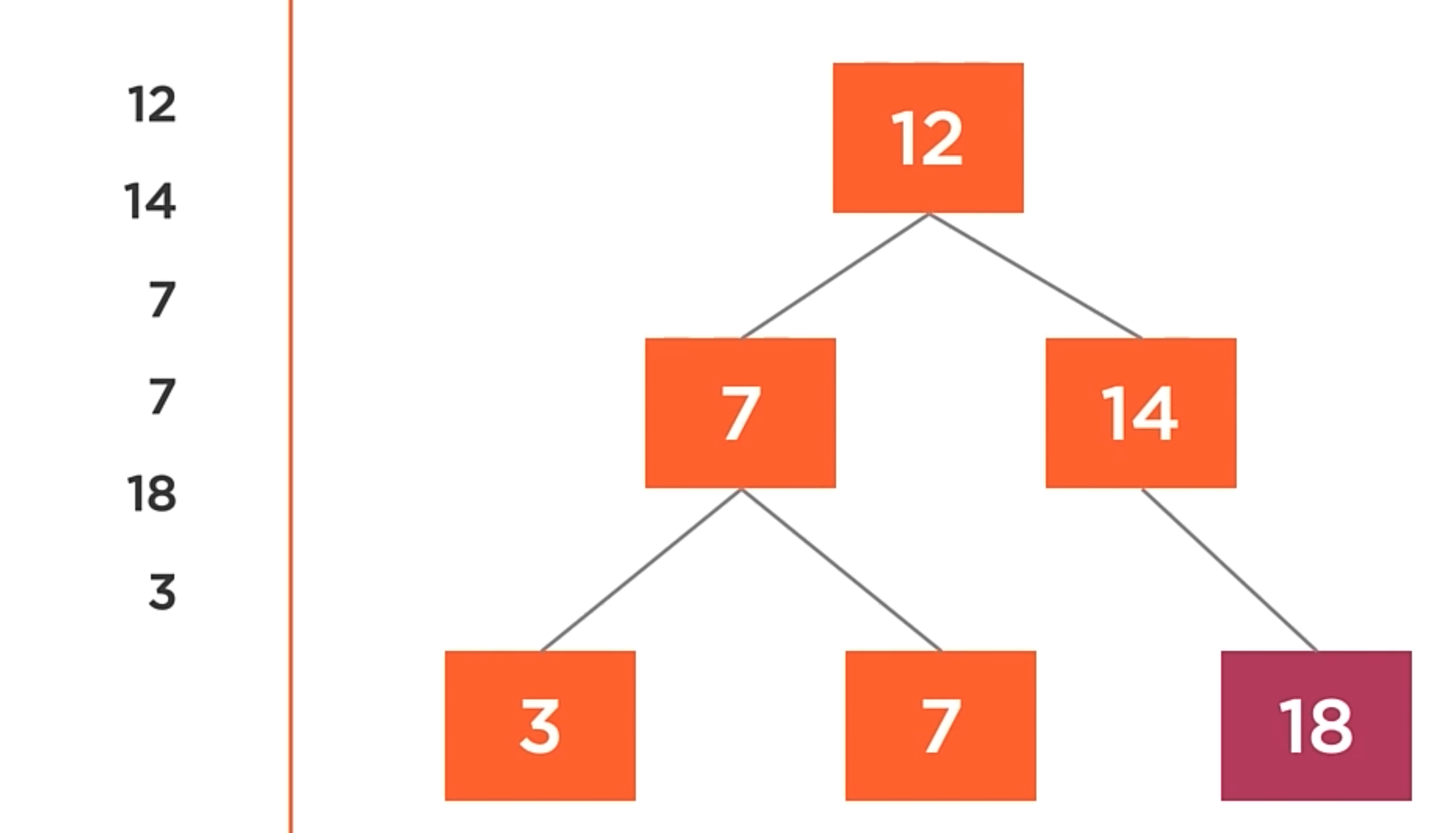
In the image below, take into account that the greatest value will be in the right. That is the main difference between a binary search tree and a binary tree.
In terms of insertion complexity, the average case will be O(log n) and the worst case will be O(n).
There is a case when the nodes interested unbalance the tree. For example, if the root node its a 3, and then insert 2 times 7 and then an 8, the tree will be unbalanced. In this case, you will need to rebalance the tree. When the tree is unbalanced, the average case will be O(n). Exist so many algorithms that can solve this problem.
Traversal Operations
The way of visiting each nodes and perform actions on them. Here we’ll use the traversal algorithms that perform the basic tree operations, they visit the left child, and then visit the right child and process the current value. The difference between the traversal algorithms is the order of those three operations is perform and how that order may impact the data we get back.
- Pre-order: The node is visited before it’s children.
- In-order: The left child is visited before the node, then the right child.
- Post-order: The left and right children are visited before the node.
Pre-Order traversal
- Process the current value,
- Visit the left child,
- Visit the right child.
All those operations are performed recursively.
1 | // Accept an action to perform when processing a node (Will be called for each node) |
In the code above, we create a method called PreOrderTraversal. This method will accept an action to perform when processing a node. The method will call the private recursive method with the Root node executing the action of the node and then checking the Left node and then the right node.
The most common scenario is to copy the tree into another.
1 | BinaryTree<int> original = new BinaryTree<int>(); |
In the code above, we create a new BinaryTree called copy. Then, we add the values to the tree
.
In-Order traversal
In this case, the order change
- Visit the left child,
- Process the current value,
- Visit the right child.
1 | // Accept an action to perform when processing a node (Will be called for each node) |
In the code above, we create a method called InOrderTraversal. This method will accept an action to perform when processing a node. The method will call the private recursive method with the Root node and first that method will check the Left node, the action of the node and then the right node.
The most common scenario is to retrieve the tree ordened.
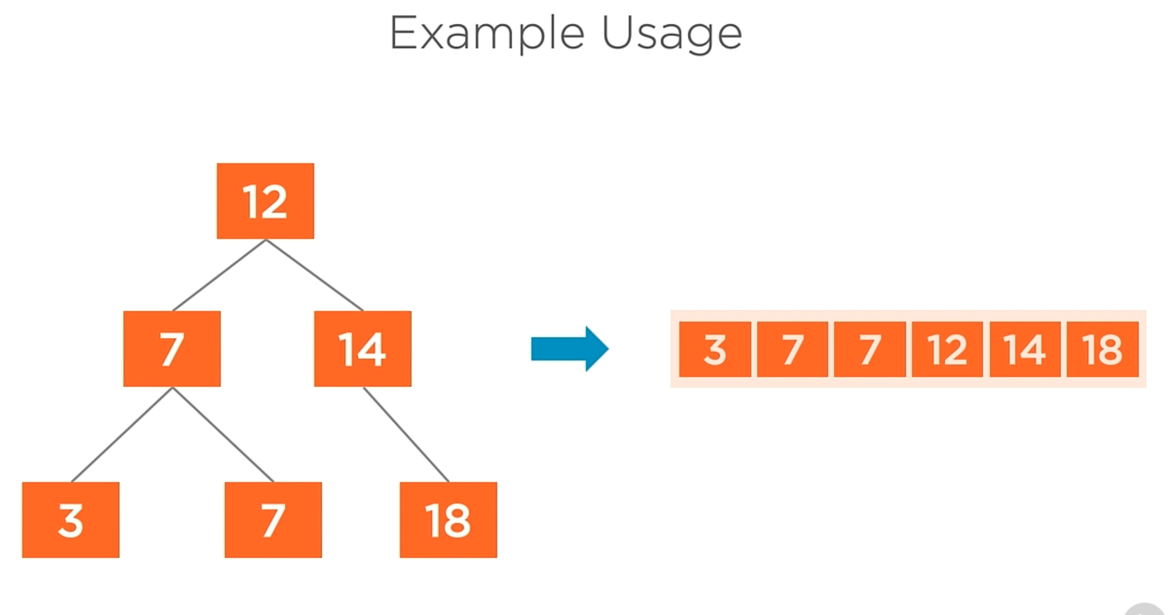
1 | BinaryTree<int> tree = new BinaryTree<int>(); |
In the code above, the In-order traversal iterates overt the nodes in sort order and print the value of each node.
Post-Order traversal
In this case, the order change
- Visit the left child,
- Visit the right child.
- Process the current value,
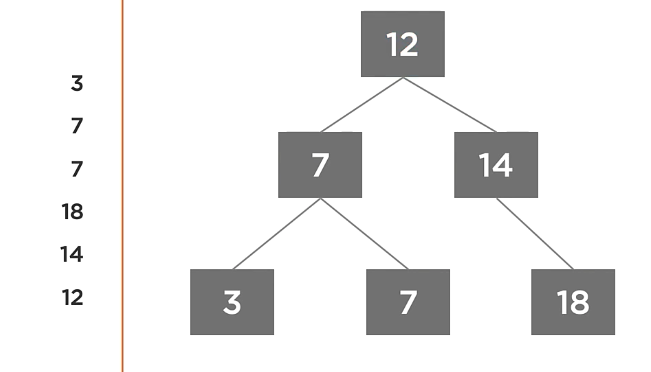
1 | // Accept an action to perform when processing a node (Will be called for each node) |
In the code above, It’s pretty similar that the previus one, but this time, the order is different. First the left child, then the right child and then execute the current action node.
The most common scenario is to delete every node in the tree. Because we need to delete the nodes first and now you can delete the parent node.
Traversal Operations Complexity
For the average case and the Worst case, the complexity is O(n). That is because in any case you need to go through all the nodes.
Search Operations
That is one of the most important topics in the tree. That is the reason why his name, Binary Search Tree.
How search operations works?
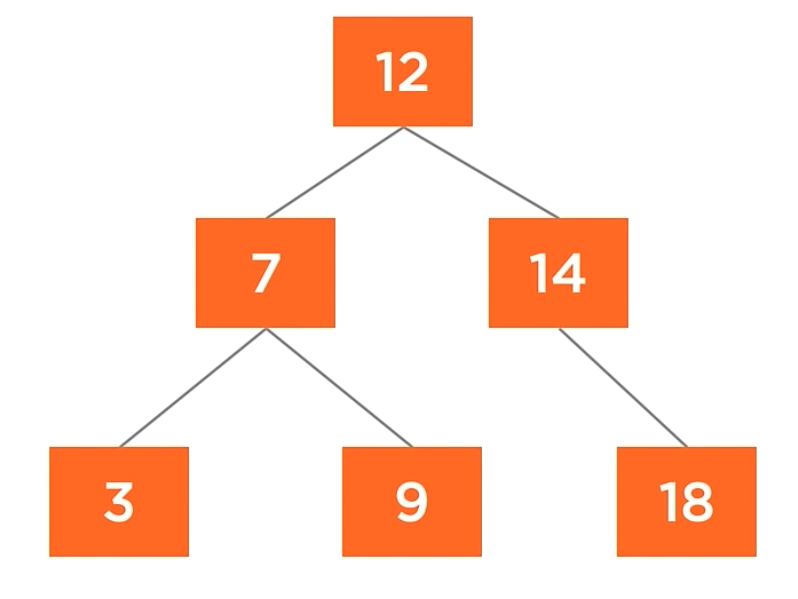
Let’s try to find the number 9 in the tree. We’ll start at the root node, which has a value of 12. We know that 9 < 12 and in a binary search tree, the smaller value always goes to the left. The good thing about this tree is that you don’t even need to go to the right node, because we know that the value is not in the right part of the tree.
Going to the left child, we find the value 7, and 7 > 9. So, we go to the right child of the node. And now we found the value with the value of 9. All this process only searching 3 nodes of the tree, skiping 50% of the tree.
The traversal complexity of the search operation is O(log n) in the average cases and O(n) in the worst cases.
Example of a Binary Search Tree
In the course, the teacher explain the difference between a SortedList and a Binary Search Tree. Inserting 25.000 records took around 60 seconds and with the Binary Search Tree, it took around a few miliseconds.
Both of them implements the IEnumerable pattern, all the code in the example that enumerates over the data will continue working. And in the tree the in-order traversal is the default enumeration order. aditionally, all the function expect sorted data.
Part of the code of the course is:
In the code above, we create a class called SortedListNode. This class is a implementation of IEnumerable.
Let’s see the implementation of the Binary Tree.
Hash Tables
The Hash tables are associative array container that provides O(1) time complexity for the operations like insertion, removal, and lookup.
1 | HashTable<String, String> headers; |
In the code above, the Hash table stores HTTP header data where the key and value are both strings.
You can use any type of data as the key and value. The important thing here is that the key must be unique.
Associative Array
A collection of Key/value pairs where the key can only exist once in the collection. They’re like arrays, but instead of indexing with integers, you can index with any data type.
Some examples of Associative array are:
HTTPS Headers.
Application Configuration File.
Environment Variables.
Key/Value database.
In all these examples, the key is the name of the variable and the value is the value of the variable.
Hash Function Properties.
The Hash function is a function that maps data of arbitrary size to data of a fixed size. The Hash function is very popular in the computer science world, the most common cases are verifying downloaded data, storing passwords in a database, or Hash tables key lookup.
For a function to be a suitable hash function, it has to have three properties.
- Stability (The hash function must always return the same result).
- Uniform Distribution (The hash function must always return the same value for a given input).
- Security (The hash function must never reveal the input).
A good example of uniform distribution is the following example:
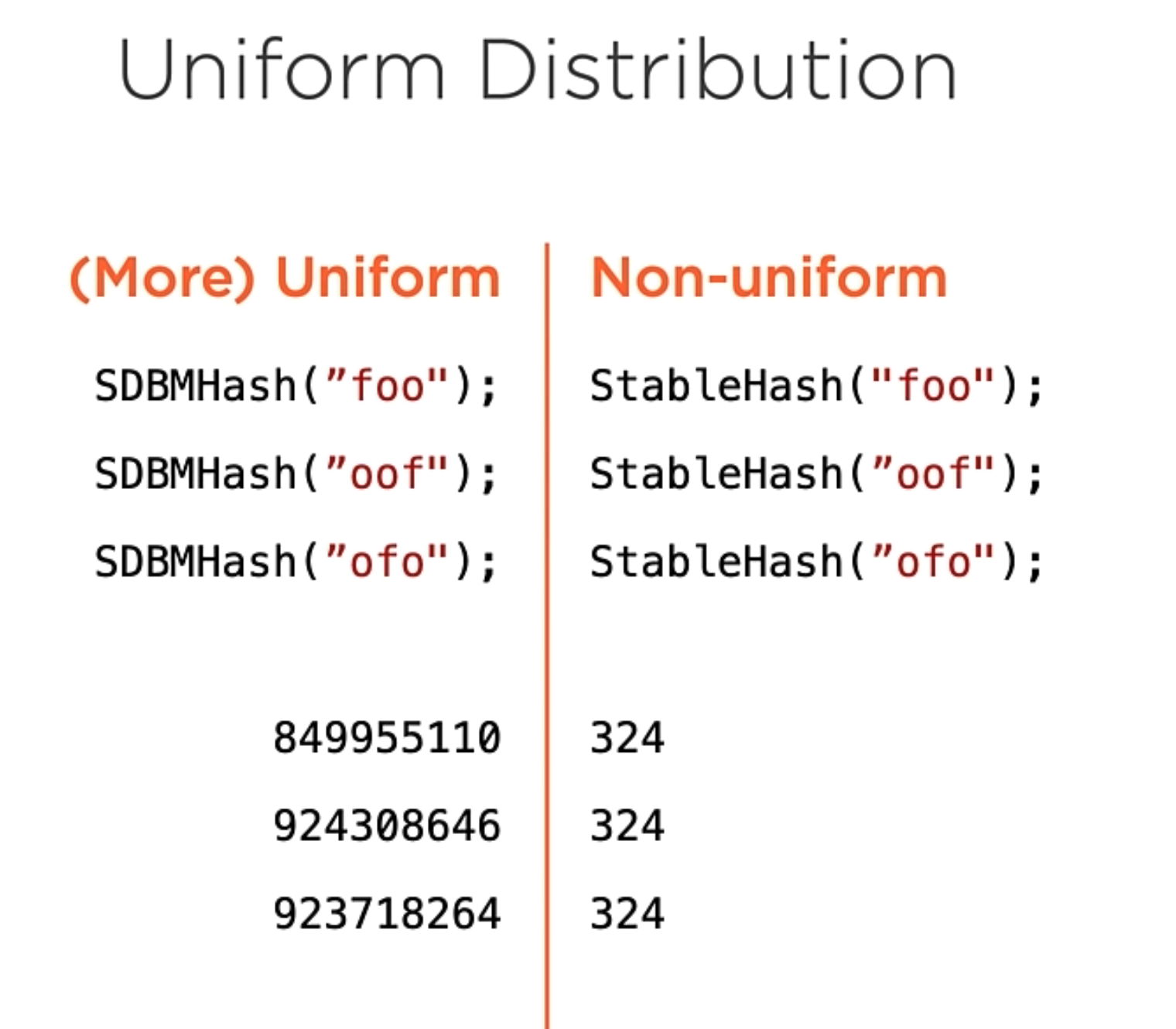
Sample Hash Algorithms
For the records, those algorithm samples a probably not appropriate for your application domain.
Additive Hash
Pros:
- Stable
- Fast
Const:
- Poor Uniformity
- Poor Security
1 | [ f | o | o ] // Original string |
This Algorithm is very simple. It’s just a simple addition of the ASCII value of each character.
Folding Hash
Pros:
- Stable
- Fast
- Better Uniformity
Cost:
- Poor Security
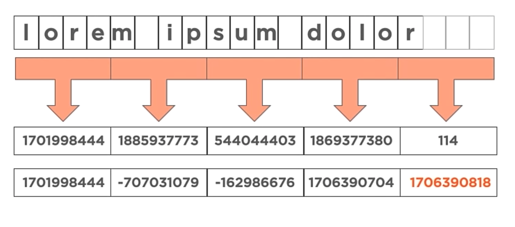
This Algorithm is pretty similar to the previous one, but instead of adding the ASCII value of each character, it combines the characters into groups of four. So, the first 4 8-bit characters are combined into a single 32-bit value, the next 4 8-bit characters are combined into a single 32-bit value, and so on.
Dbj2 Hash
This algorithm is an implementation of the additive hash and it’s being altered to be more secure and with better uniformity.
1 | public ulong Dbj2Hash(string input){ |
This algorithm is a better implementation of the previous one because it’s more secure and with better uniformity. Altering the Hash calculation avoids being predictive.
Hash function comparison
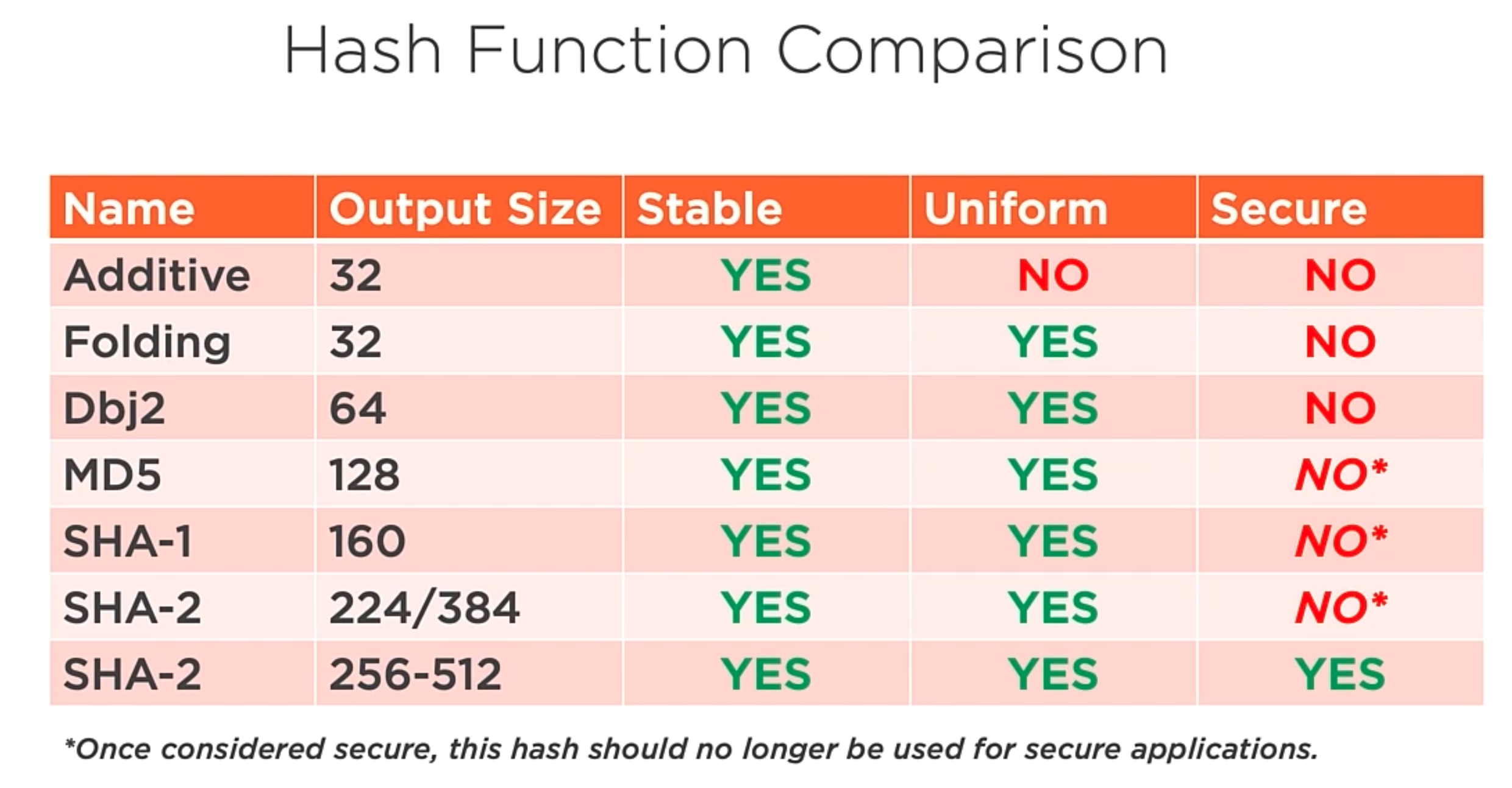
Several of these algorithms were considered secure at one point, but due to the computational increase, they are no longer safe.
Hash Tale Operations
There are several operations that can be performed on a Hash Table. Let’s see them.
Add
1 | // key and value type parameters |
In the code above, the HashTable class receives the key and value type parameters. Additional has a function to support indexed get and set operations using the key type.
Hash Collision
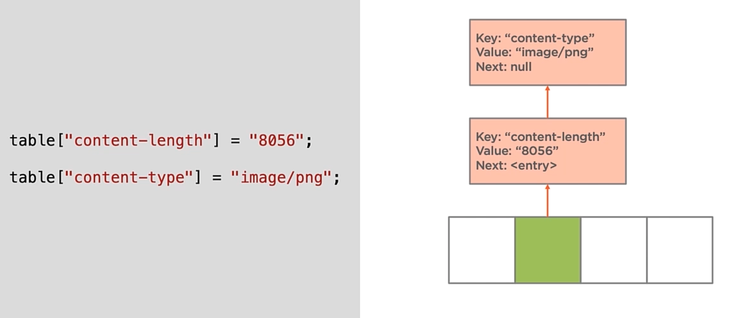
A hash collision occurs when multiple distinct keys will be inserted at the same hash table index. As you saw earlier, the index function is a function that calculates the Hash of the key and then modulo the length of the table. So, if the table has a length of 4, the index function will return the index of the table where the key will be inserted.
So, there is a technique to handle that type of collision. The Separate Chaining technique is used.
- The Collisions in a hash table are chained together into a linked list whose root node is the hash table array entry.
1 | internal class HashTableentry<TKey, TValue> |
The HashTableentry class is a node of the linked list.
With this example, when there is a collision, the new item will be inserted in the LinkedList.
Insertion
In the Hash tables, As more items are added, the remaining indexes begin to be filled. And Eventually, every array index of the table will contain at least one item. As this happens, the number of collisions will increase. So, if the goal of the Hash tables is to have O(1) or constant time operations, it’s hard to handle that time when the array is full of linked lists. And Every Linked List has an O(n) time complexity.
When there are so many collisions, it’s time to think that maybe the array is too small. There is a way to measure that and is the following topic.
Fill Factor
The percentage of capacity representing the maximum number of entries before the tale will grow. E.g. 80% of the capacity.
E.g. If an array has 100 indexes and a fill factor of 80%. Then once the hash table contains 80 items, the array needs to grow.
Growth Factor
The multiple to increase the capacity of the hash table when the fill factor has been exceeded.
- E.g. 1.5.
Hash table Growth
There are several steps to determine if you need to grow the hash table.
- Use the fill factor to determine if growth is needed.
- Use the growth factor to allocate a larger array.
- Determine the new index for the existing items in the hash table.
- Update the hash table to use the new array. You need to iterate through the old array and re-insert the items into the new array.
Iteration
NOTE: The hash table never is going to guarantee the order of the items.
Items are iterated in the order they are stored in the table. To iterate the table you need to follow the next steps:
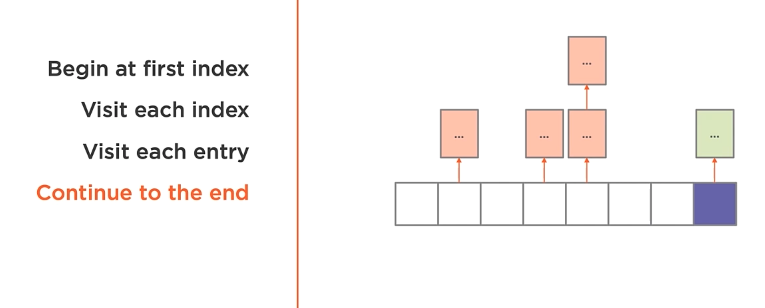
Search
Maybe one of the biggest advantages of the Hash Table is the search operation. The search operation is O(1) in the average case and O(n) in the worst case.
Finding items in the hash table become trivial. You simply find the index in the array that matches the provided key, and then we iterate the linked list looking for the entry that has the key.
- Find the index
- Use the hash function
- Modulo the hash
- Search the entry list.
Removing the items
- Determine the index
- Search the entry list
- Remove the entry.
Real Use Case of Hash Tables
In the demo of the course, the teacher adds State-level caching. The idea is to make filtering by state faster.
1 |
|
In the code above, the ContactStore class has a HashTable that stores the contacts by state. The Methods Search, remove and Add are the only methods that use the state-level cache.
Sorting and searching array data structures
What is sorting?
Well, let’s take a look into the following unsorted array of integers.
1 |
|
It’s unsorted because the values in the array are not being stored in numeric order. To sort the data, we need to move the values in the array to the correct position. The smallest values are moved to the left and the largest values are moved to the right.
Measuring Performance
When we measure the performance of a sorting algorithm, there are two important things to consider.
- Comparisons: When two values in the array being sorted are compared for relative equality.
- Swaps: When two values in the array being sorted exchange positions.
When we measure the performance of a sorting algorithm, we’re expressing the cost using Big-O notation. The actual cost of either operation depends on multiple factors. So, reducing ether operation can improve the performance.
Array sorting algorithms
General sorting algorithms:
Bubble Sort:
The basic algorithm for bubble sorting is:
- Iterate: Iterate each item over the array from start to end.
- Swap: If any two neighboring elements are not in sort order, swap them.
- Repeat: Repeat until the array is sorted.
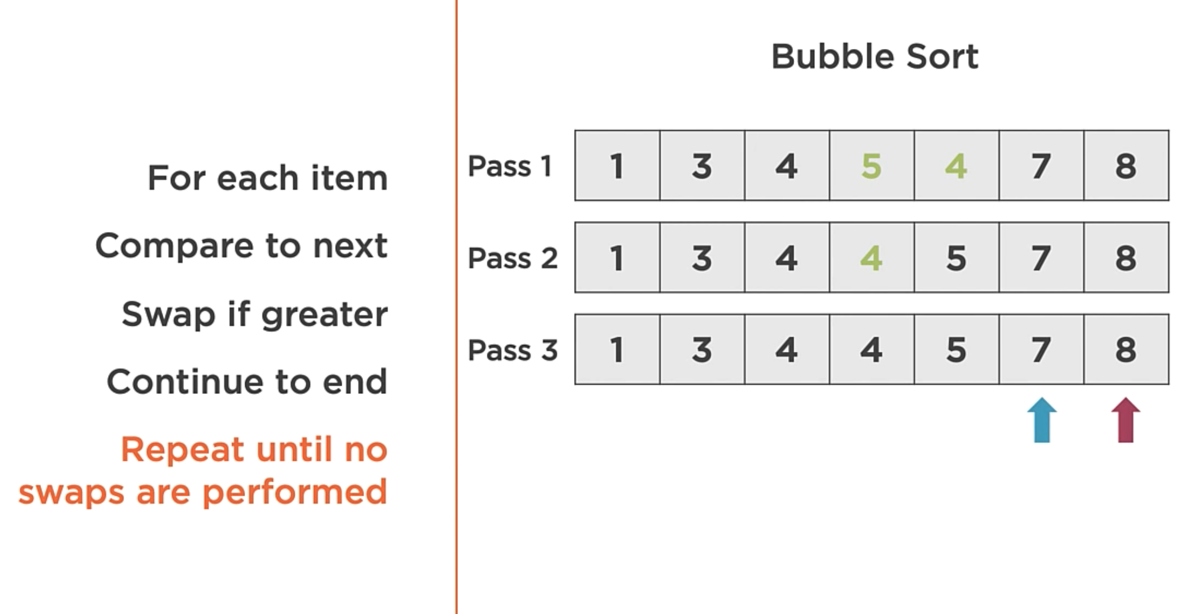
In the image above, the algorithm order the array with only 3 passes through the array.
Bubble Sort Asymptotic Analysis.
- Best: O(n) comparisons and swaps
- Average: O(n^2) comparisons and swaps
- Worst: O(n^2) comparisons and swaps
Having an average of O(n^2) makes it a poor general-purpose sorting algorithm.
Insertion Sort
The Insertion Sort algorithm does the following:
- Iterate: Iterate each item over the array from start to end.
- Compare: Find out of order neighboring items. When the out-of-order item is found, instead of swapping with the neighbor element (Like the bubble sort does),
- Shift and Insert: Find the insertion point, shift, and insert into the correct position.
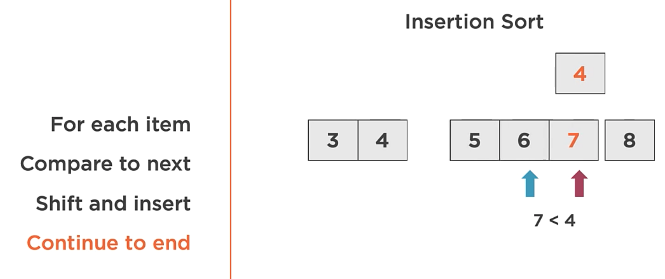
In the image above, the algorithm order the array with only 1 iteration through the array.
##### Insertion Sort Asymptotic Analysis. - Best: **O(n)** comparisons and swaps - Average: **O(n^2)** comparisons and swaps - Worst: **O(n^2)** comparisons and swaps
Despite the average case of O(n^2), the Insertion Sort can be useful in specific cases.
Insertion Sort use cases
- Adaptive: So, it works well when the data is nearly sorted.
- In-place: Requires only O(1) additional memory.
- Online: Sorting can occur as the data is received. So, it’s useful for streaming data and it does not need to have the entire array in memory.
Merge Sort
This one is a bit different from the previous two. The basic algorithm follows the rule of divide and conquers approach.
- Divide: Split the array into sub-arrays of a single item.
- Compare: Compare the individual items.
- Merge: Merge the items into a sorted array.
That may sound a little confusing. So, let’s take a look at the following example.
1 | // Here is the initial array |
Merge Sort Asymptotic Analysis.
- Best: O(n log n) comparisons and swaps
- Average: O(n log n) comparisons and swaps
- Worst: O(n log n) comparisons and swaps
The merge sort algorithm is a stable sorting algorithm. It has a uniform algorithmic complexity in the worse, average, and best case.
Some of the properties of merge sort:
- Divide and conquer: reduces the problem down to the most basic form.
- Memory requirements: Requires only O(n) additional memory.
- Stable: Equal items retain their relative position.
Quick Sort
The QuickSort algorithm it’s another divide and conquers algorithm, but it with a different approach. It does the following:
- Pivot: Pick the pivot value in the array.
- Partition: reorder the elements around the pivot point.
- Repeat: Repeat for each partition.
The pivot value
The pivot value is a value in the array where all the values to the left of the pivot are less than (Or equal to) the pivot value, and all the values to the right are greater.
How to select a pivot value:
- Random: Pick a random value in the array.
- Median of three: Pick the median of the first, middle, and last values in the array.
- First or the last item: Pick the first or the last item in the array.
Warning: Selecting the first or the last value in the array is not a good choice. If the array is presorted, and then picking this value as the pivot value will cause the algorithm to be O(n^2). Which is not disarible in a general-purpose sorting algorithm.
Partitioning
After the pivot point has been selected. We need to partition the array around the pivot point. So, all the values on the left of the pivot point are less than (Or equal to) the pivot value, and all the values to the right are greater.
E.g.
1 | [ 9 | 6 | 4 | 3 | 8 | **5** | 4 | 1 | 2 | 6 ] |
Quick Sort Asymptotic Analysis.
- Best: O(n log n) comparisons and swaps
- Average: O(n log n) comparisons and swaps
- Worst: O(n^2) comparisons and swaps
Quick Sort properties
- Divide and conquer: reduces the problem down to the most basic form.
- In-place: Requires only O(log n) additional memory.
- Optimizable: There exist many optimizations to improve the performance of the algorithm.
Due to this fact, the Quick Sort is the default sorting algorithm for many programming languages.
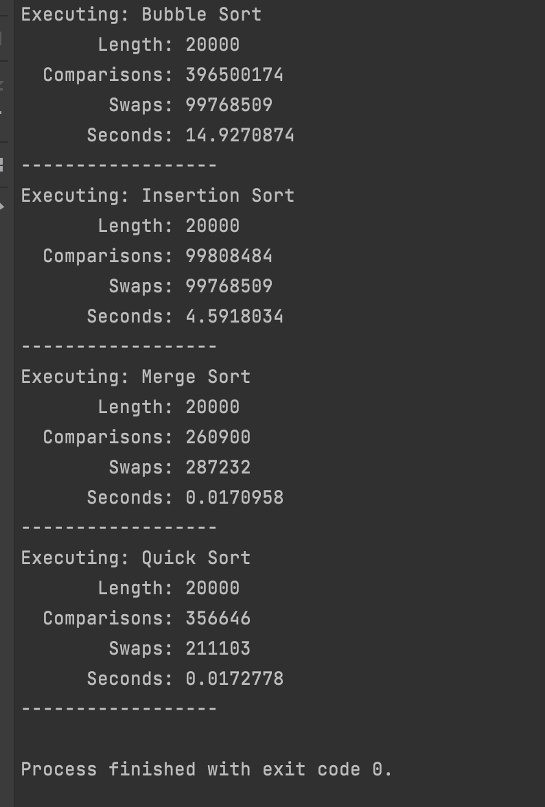
Sorting algorithms Comparison
This is the comparison between all the sorting algorithms with 20.000 records.
Searching array data
Now that we already know how to sort the array of data let’s see how to search for a value in an array and how
sorting can help make that more efficient.
Linear Search
Scan the array, from start to end, comparing each array item against the value being sought. It’s pretty straightforward to implement:
1 | public bool Search(int[] array, int value){ |
The Asymptotic analysis of this algorithm is O(n). That is because it needs to scan each item in the array until the value has been found.
Binary Search
If the linear search algorithm consists in searching in an unsorted array, the binary search algorithm starts with a sorted array. It’s like searching in a dictionary, in which every word is stored alphabetically.
So, starting with a sorted array, check the middle array value. If the value is a match, then the value has been found. If the value is greater than the sought value, repeat this process for the values to the left, otherwise for the values to the right.
1 | //Search the value 2 into the following array. |
Now let’s see a binary sort implementation.
1 | public bool BinarySortSearch(int[] data, int value){ |
This algorithm is O(log n). It’s because it needs to divide the array in half until it finds the value.
Although, this algorithm is very efficient for searching in a sorted array, but don’t assume that this means that you should always sort data before searching. Linear search is an O(n) operation, but if the data is unsorted, sorting the data will be more expensive than simply performing a linear search.
String Searching Algorithms
Disclaimer: In this module, the search algorithms will be classes that implement the IStringSearchAlgorithm interface.
The IStringSearchAlgorithm defines the function, Search, which will be called to find all of the matches of the search string (pattern) within the input (toSearch) string.
1 | public interface IStringSearchAlgorithm |
Example usage
The search method of the IStringSearchAlgorithm instance (algorithm) returns each of the matches as an enumeration of ISearchMatch objects.
1 | string pattern = "fox"; |
Naive String Search
1 |
|
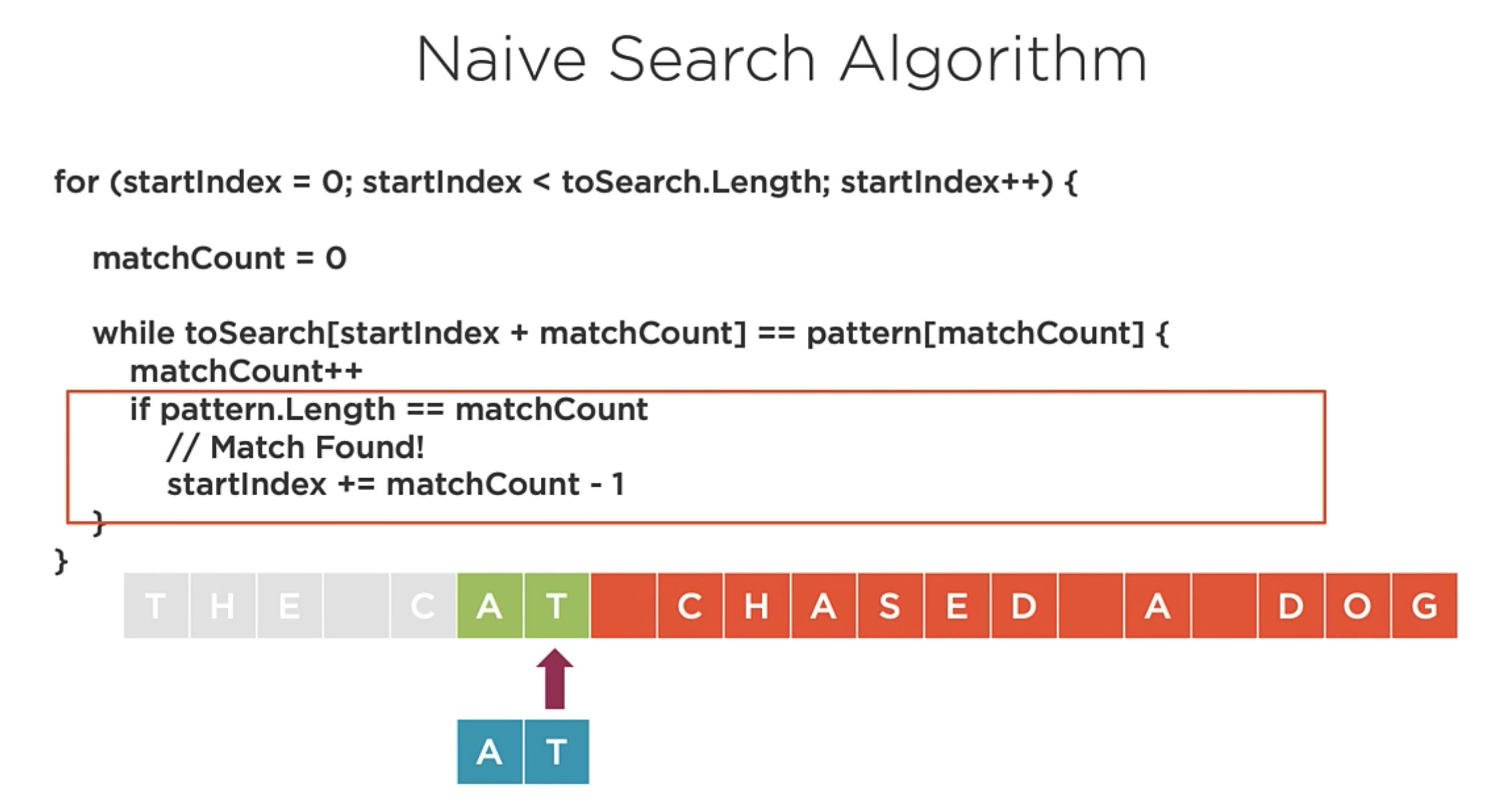
Naive String Search Asymptotic Analysis
Average: O(n + m)
Worst: O(nm)
No requires pre-processing of the data. Appropriate for small inputs.
Boyer-Moore-Horspool String Search
It’s a 2-stage search algorithm that use a table that contains the length to shift when a bad match occurs.
First Stage
Pre-process the string to find to build a bad match table.
Second Stage
The string to find is search right-to-left using the bad match table to skip ahead at a mismatch.
The code Example
1 | class BadMatchTable { |
In the code above, the BadMatchTable class is used to build the bad match table.
1 | // Construct the BadMatchTable with the pattern to search. |
| Index | Value |
| —– | —– | —————————————————————– |
| ? | 5 |
| T | 4 | pattern.Length (5) - i (0) - 1; |
| R | 3 |
| U | 2 |
| T | 1 | // Update T with the offset of the last character in the pattern. |
This means if we compare the last character of the string, H, and we find a T, instead of sliding forward the length of the string, It will only slide forward 4 characers. This will align the T’s and allow us to verify if we have a match.
1 | // Searching the string TRUTH in the array. |
Boyer-Moore-Horspool Performance
- Average: O(n)
- Worst: O(nm)
The larger the bad match table, the better the performance.
Code Implementation for Boyer Moore horspool.
Balanced Binary Trees
Binary Search Trees
A sorted data structure where each node can have 0-2 children, and each node, except the root, has exactly one parent.
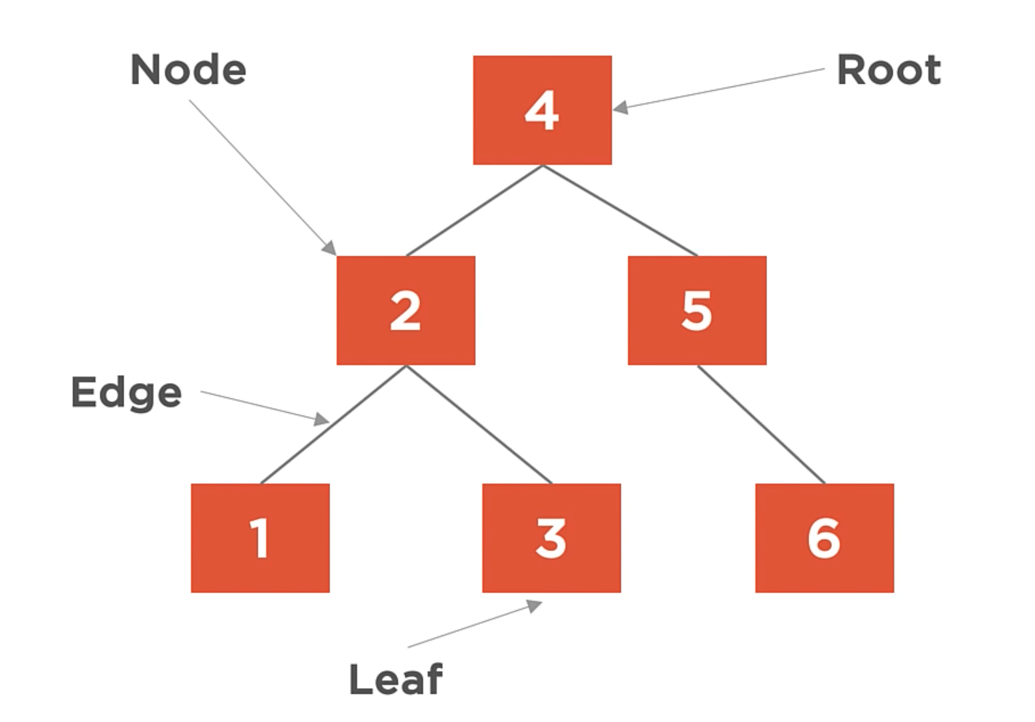
In a binary search tree, values are stored in a specific order. Smaller values are stored on the left, and larger values are stored on the right.
It means that the binary Tree insert, remove and search operations are O(log n) average case. Unless the tree is very unbalanced, which is very rare.
Unbalanced Tree
It’s when a tree whose left and right children have uneven heights. And the Height is the maximum number of edges between the tree’s root and any leaf.
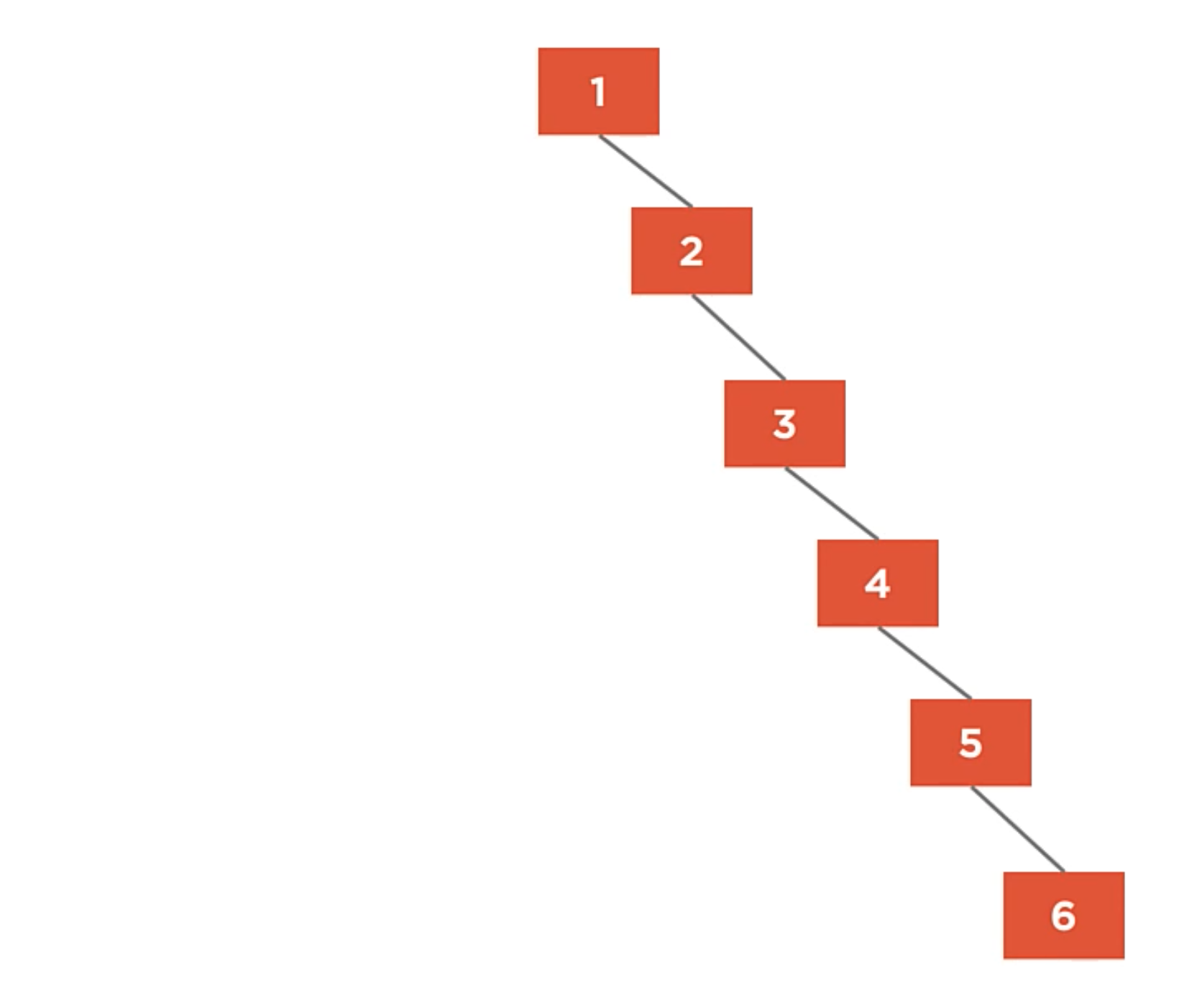
It looks more like a linked list instead of a tree. Despite following all the rules.
A fully unbalanced binary tree is just a linked list with O(n) algorithmic complexity.
Balanced Tree
It’s when a binary search tree whose maximum height is minimized. In the example below, each of the leaf nodes has a maximun of height is 2.
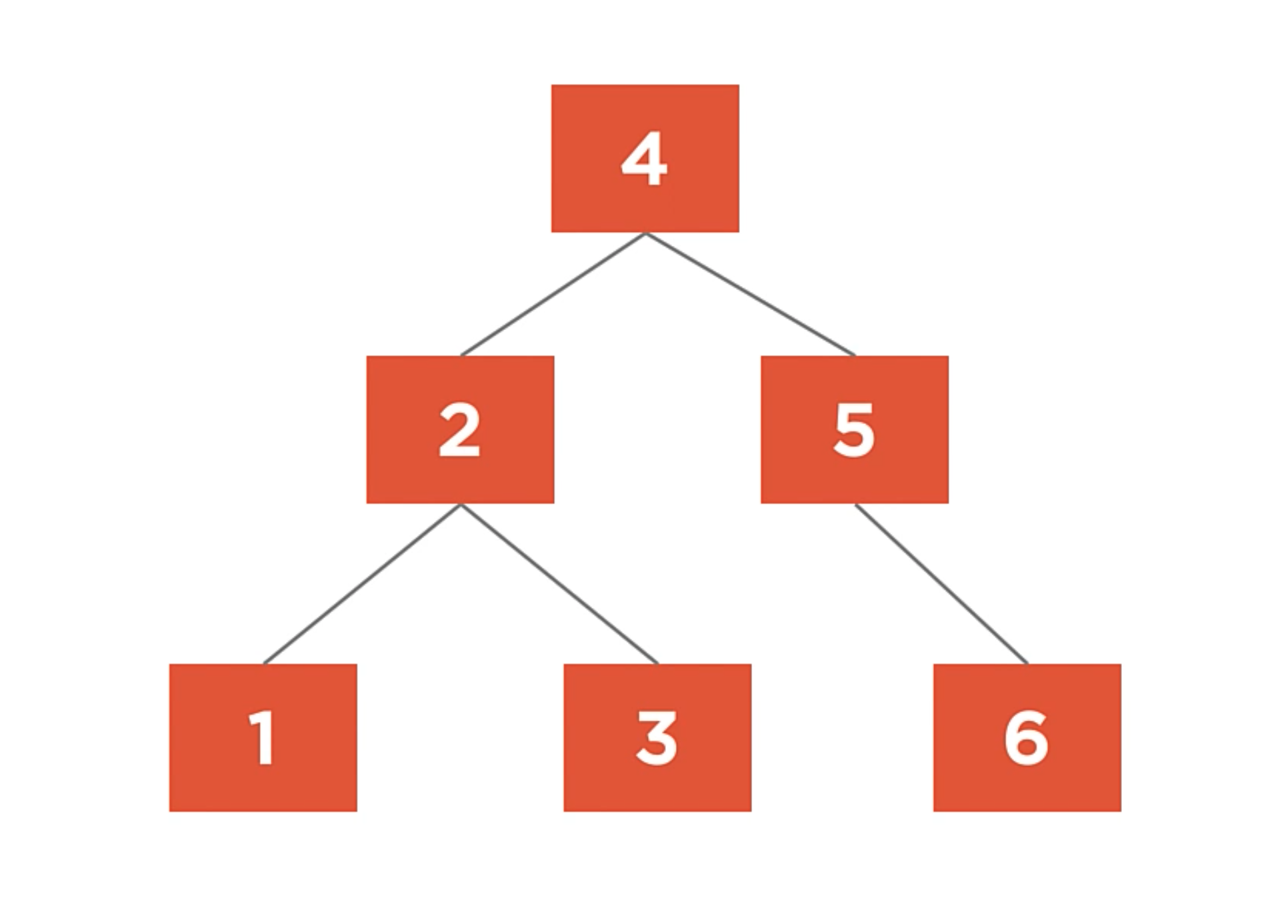
Balance Factor
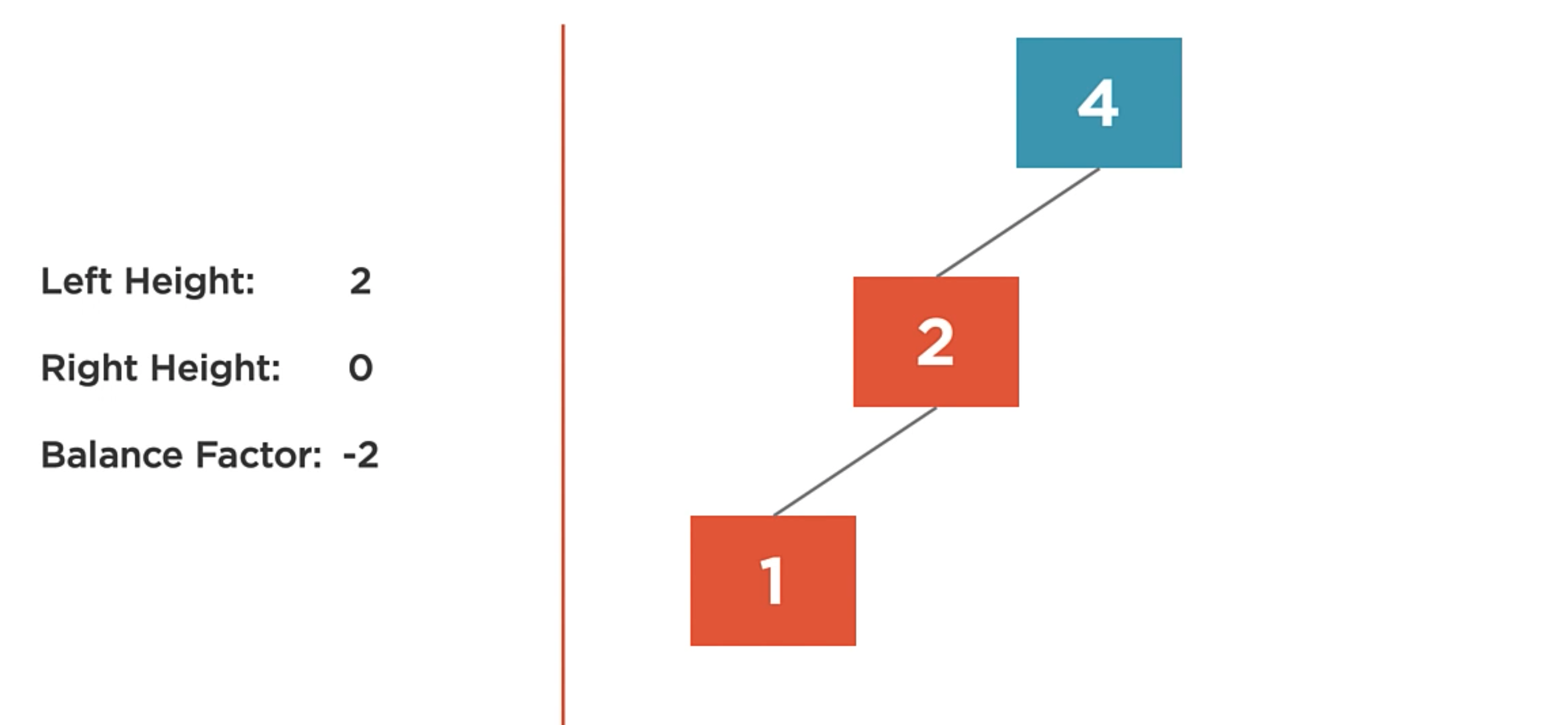
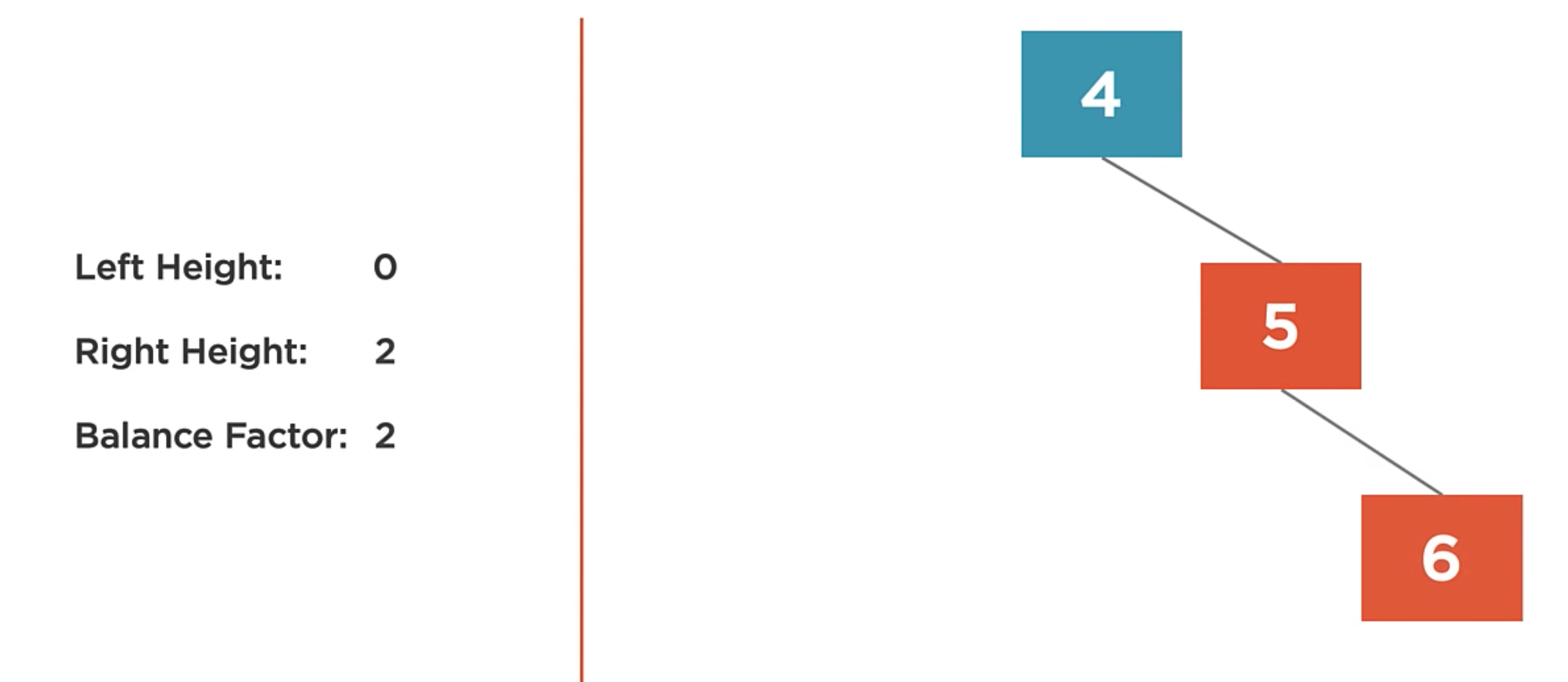
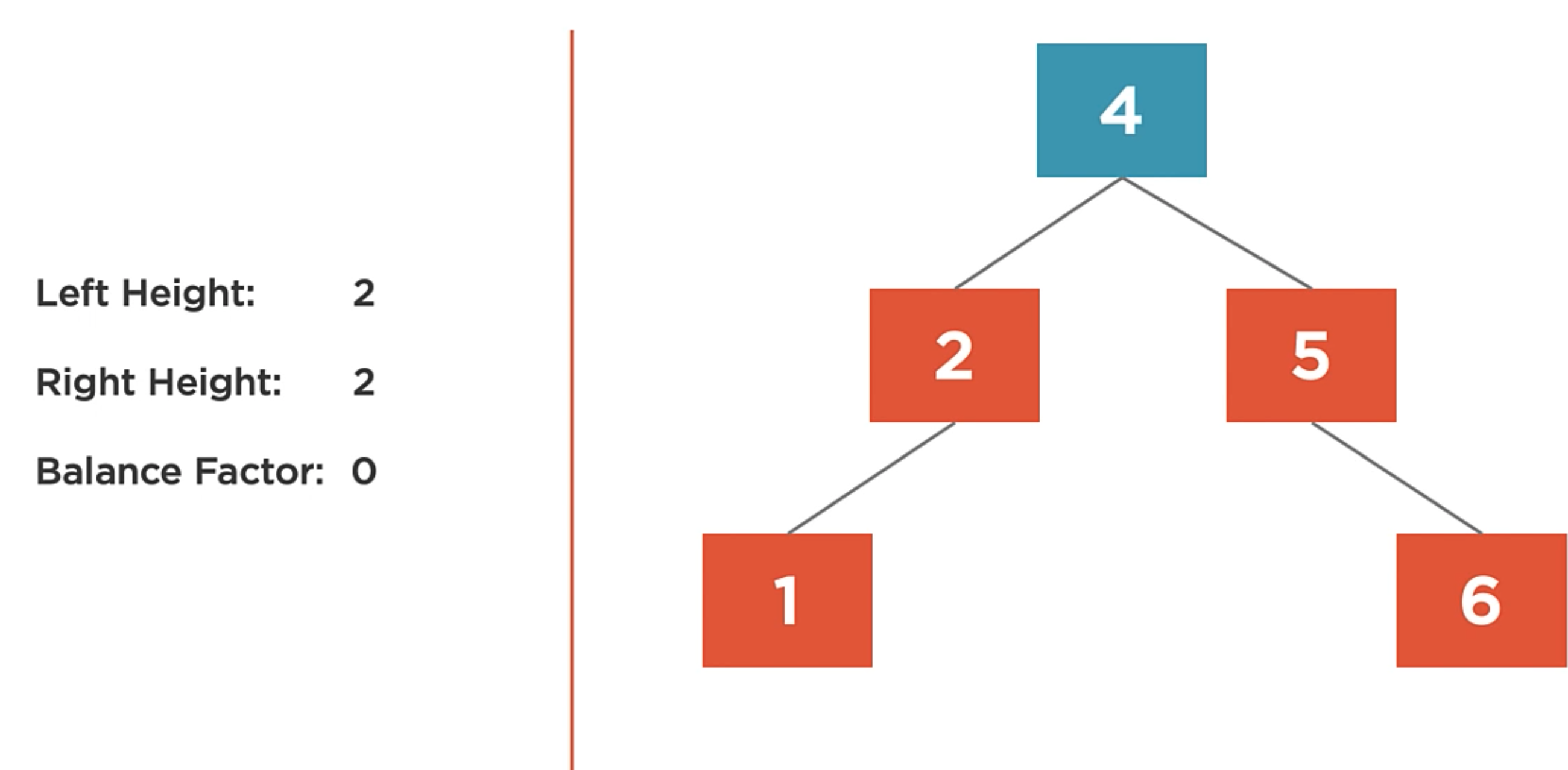
The balance factor of a node is the difference in height of the left and right subtrees. We can say that the balance factor is the height of the right child minus the height of the left child.
It’s Heavy the state when the balance factor of a node differs by more than one. So, when it’s heavy, it is unbalanced.
In the following case, there is a balance factor of -2. It means that the left subtree is 2 levels deeper than the right subtree.
In the following case it is the opposite, there is a balance factor of 2. It means that the right subtree is 2 levels deeper than the left subtree.
And finally, the balance factor of a tree is 0. It means that the left and right subtrees are the same height.
AVL Tree
The AVL tree is a self-balancing binary search tree. It is a type of binary search tree that is very efficient at insertion and deletion. Named after its inventors Greorgy Adelson-Velsky and Evgenii Landis.
Self Balancing
The tree is balanced as nodes are added and or removed from the tree.
The AVL tree uses four different rotation algorithms to balance the tree.
- Left Rotation
- Right Rotation
- Left-Right Rotation
- Right-Left Rotation
The Left and right rotations are used to balance trees that are respectively heavy on the left and right.
The Left-Right and Right-Left rotations are combinations of the Left and right algorithms that are used when a single left or right rotation will not successfully balance the tree.
Left Rotation
The left rotation algorithm is used to balance a right-heavy tree by rotating nodes to the left.
- Right Child becomes the new root.
- Left child of the new root is assigned to the right child of the old root.
- Previous root becomes the new root’s left child.
Here is an example:
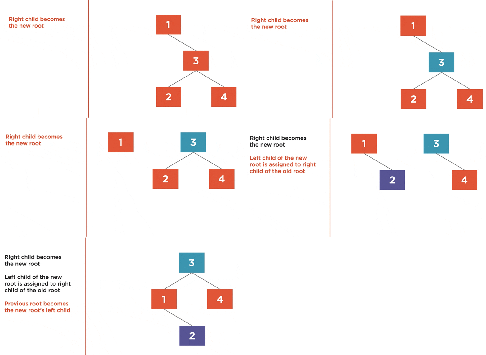
Here we have a tree with a balance factor of 2. So, it’s right heavy, and it needs to be rotated to the left.
1 | private void LeftRotation(){ |
Right Rotation
The right rotation algorithm is used to balance a lefty-heavy tree by rotating nodes to the right.
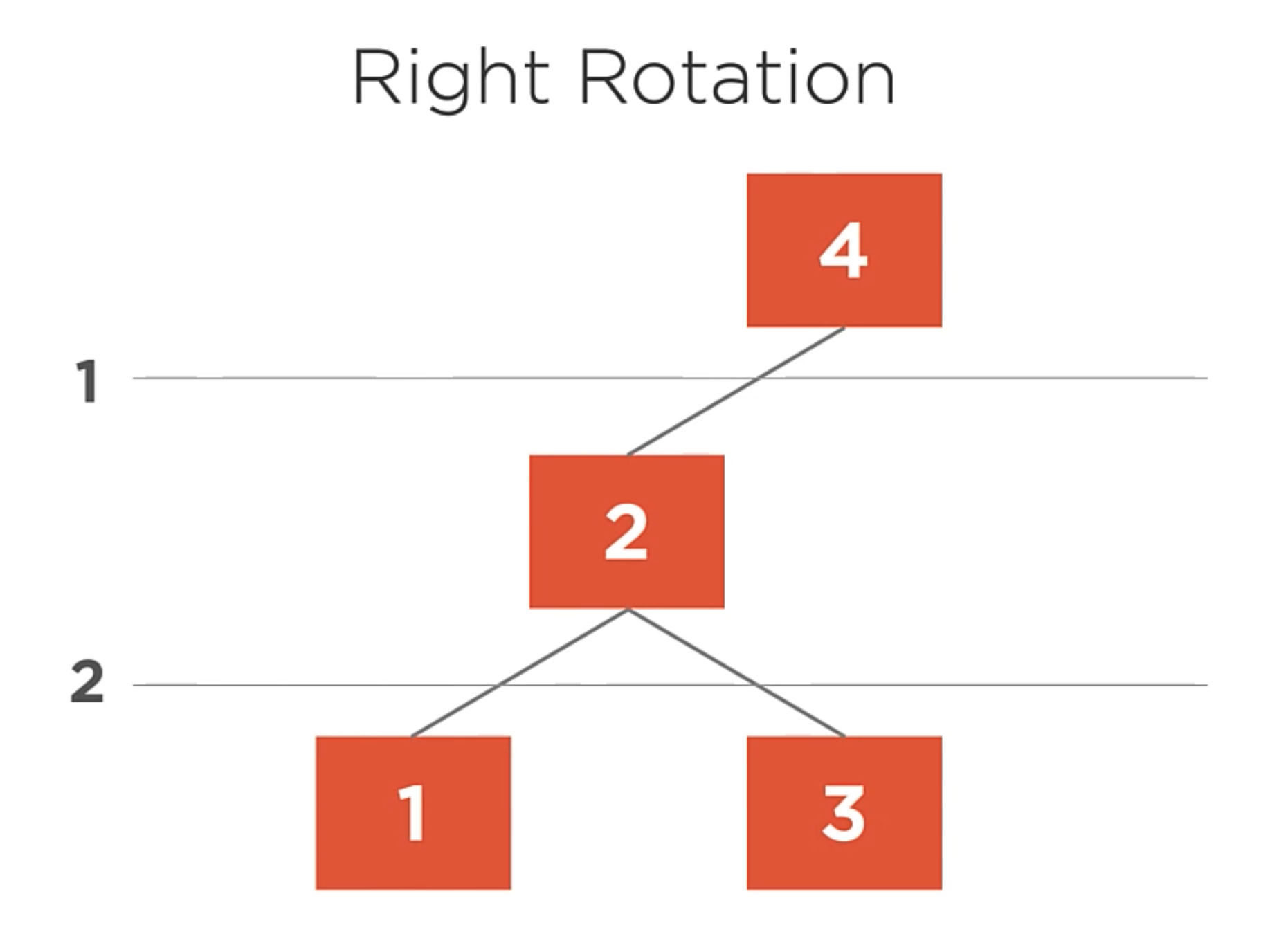
In this example, here we have a heavy tree with a balance factor of -2. So, it needs to be rotated to the right.
- Left Child becomes the new root.
- Right child of the new root is assigned to left child of the old root.
- Previous root becomes the new root’s right child.
1 | private void RightRotation(){ |
When right and left rotation are not working.
There are some cases where the left and right rotations are not working.
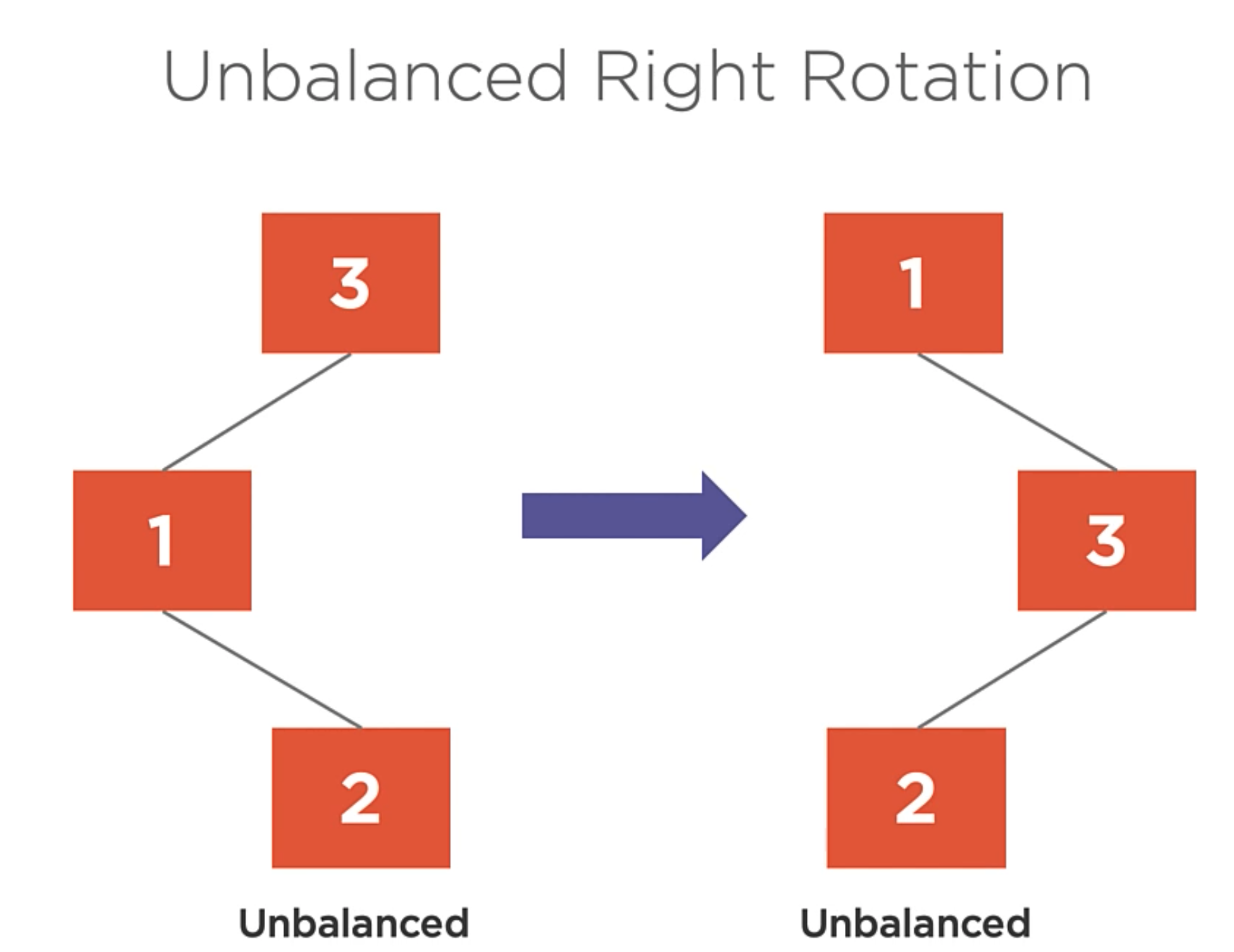
So, when you apply Right rotation into the previous example, you get the same problem but inverted.
In this case, the left-right rotation is used to balance the tree.
Right-Left Rotation
- Left rotate the left child.
- Right rotate the root.
Here is an example:
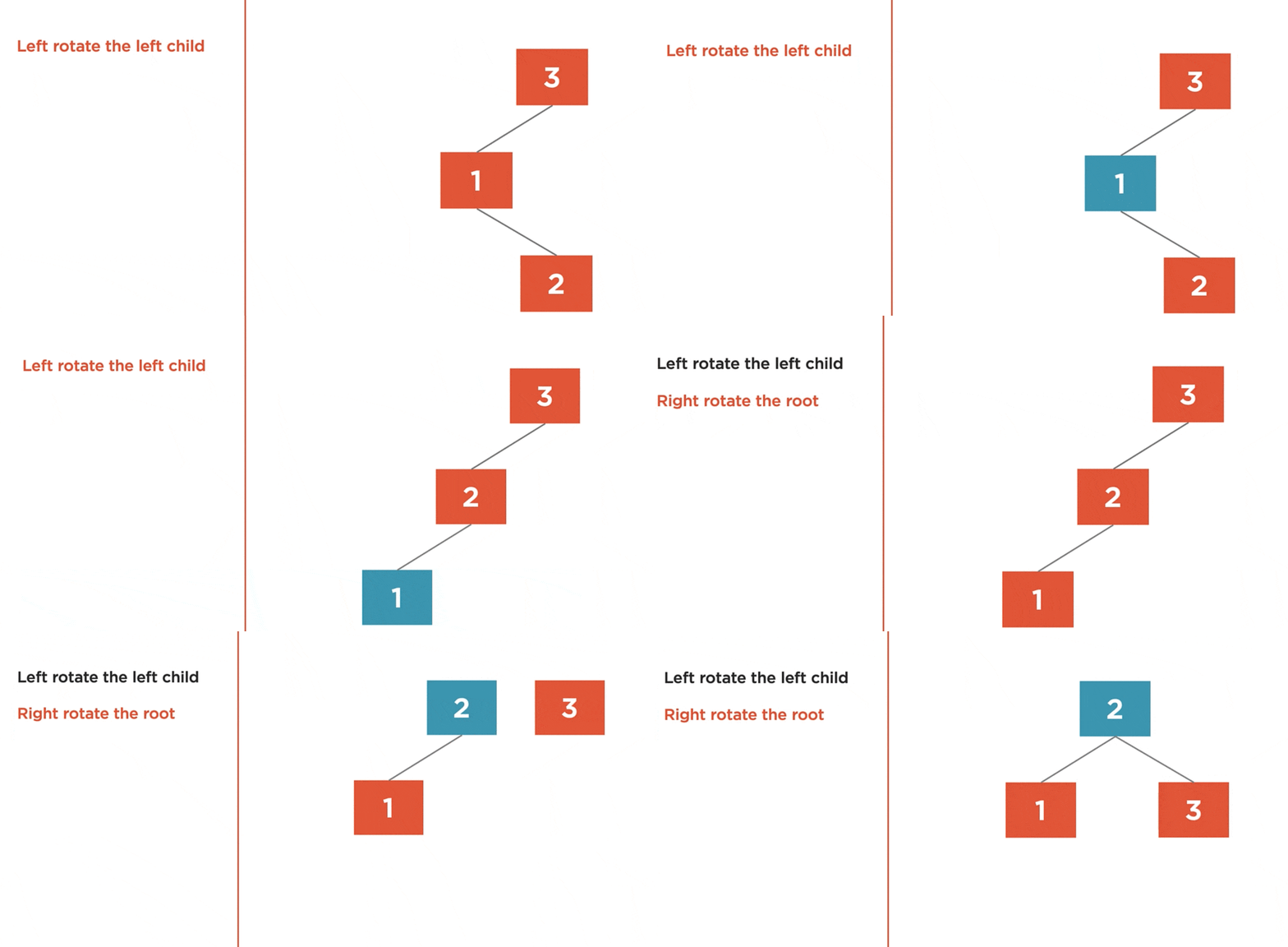
We can solve the problem with the same algorithm but inverted in the case of the left-right rotation.
The big question here is. Which rotation should be used to balance the tree?
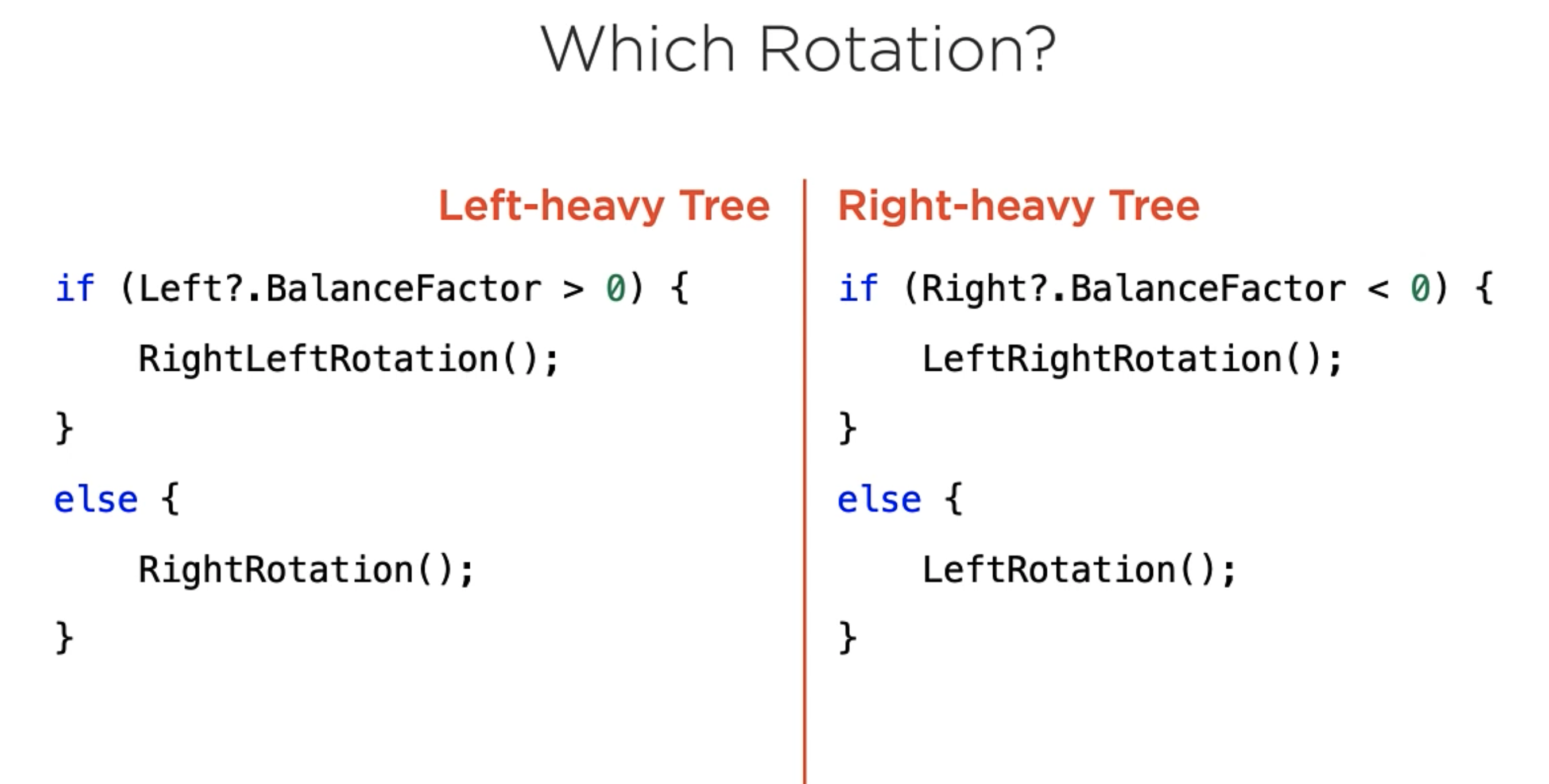
Code Examples
Here is the Tree Node class:
Here is the AVLTree class:
Sets and set Algorithms
Set
A set is a data structure that stores unique values in an undetermined order.
Set Properties
Contains only distict items: A set can hold any number of values. But any specific value can only appear within the set once. If you attempt to add a second instance of that value, the set will remain unchanged.
- For example, we could have a set of integers 1 through 10. If we try to add the integer 1 again, the set will remain unchanged.
**Items are iterated in an implementation-defined order. **
The set data structure does not define what order the items are stored in; however, your specific implementation may choose to.- For example, if your implementation uses a balanced binary search tree, such as an AVL tree to store the contents, then it would be possible to access the values of the set in sorted order by using an in-order traversal of the tree.
- However, if your implementation used a hash table, then the values would not be in a well-defined order and the order might change as the hash table changes.
Set operations are O(log n).
- No matter what the backing storage type is, sets should have O(lgn n) time for insert, search, and delete algorithmic complexity. Our set type will ensure this is true by using a balanced binary search tree as our backing store.
Set Examples:
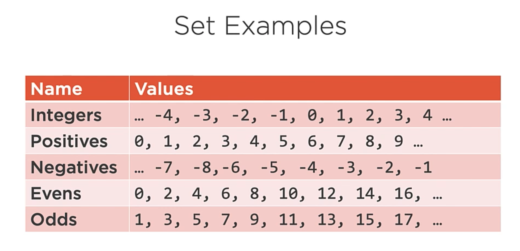
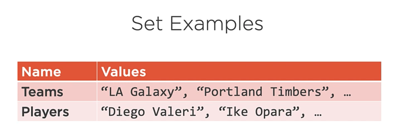
Set Code implementation
1 | // ISet implementation uses IEnumerable<T> to allow for iteration. |
In the code above, we have an ISet interface if IEnumerable. We can add, remove, and some algebra operations.
1 | public class Set<T> : ISet<T> where T : IComparable<T> |
In the code above, we have our Set class that implements the ISet interface. When the set is created, we allocate the empty AVL tree. Also, there is a constructor that takes an IEnumerableas an argument.
1 | public bool Add(T item){ |
In the code above, we have the Add method. This method adds an item to the set if it is not already in the set. If the item is already in the set, the set is unchanged.
Others Methods
1 | public bool Contains(T item){ |
The contains, remove and count methods defer to the AVL tree’s methods.
And Finally,
1 | public IEnumerator<T> GetEnumerator(){ |
The GetEnumerator method defers to the AVL tree’s GetEnumerator method. The important thing to note here is that the AVL tree defaults to in-order to traversal, so even though sets don’t require a specific ordering of values, our set will enumerate them in order due to how its underlying store works.
Algebra of Sets
What we’ve seen so far is a Set that is simply a thin wrapper over an AVL tree class and that does not allow duplicate values to be added. On its own, this is not very interesting. What makes a Set really useful is being able to apply set algebra operations to sets.
Example: Creating a set of Teams
We initialize the set type and add the teams to the set into a MLS Teams set.
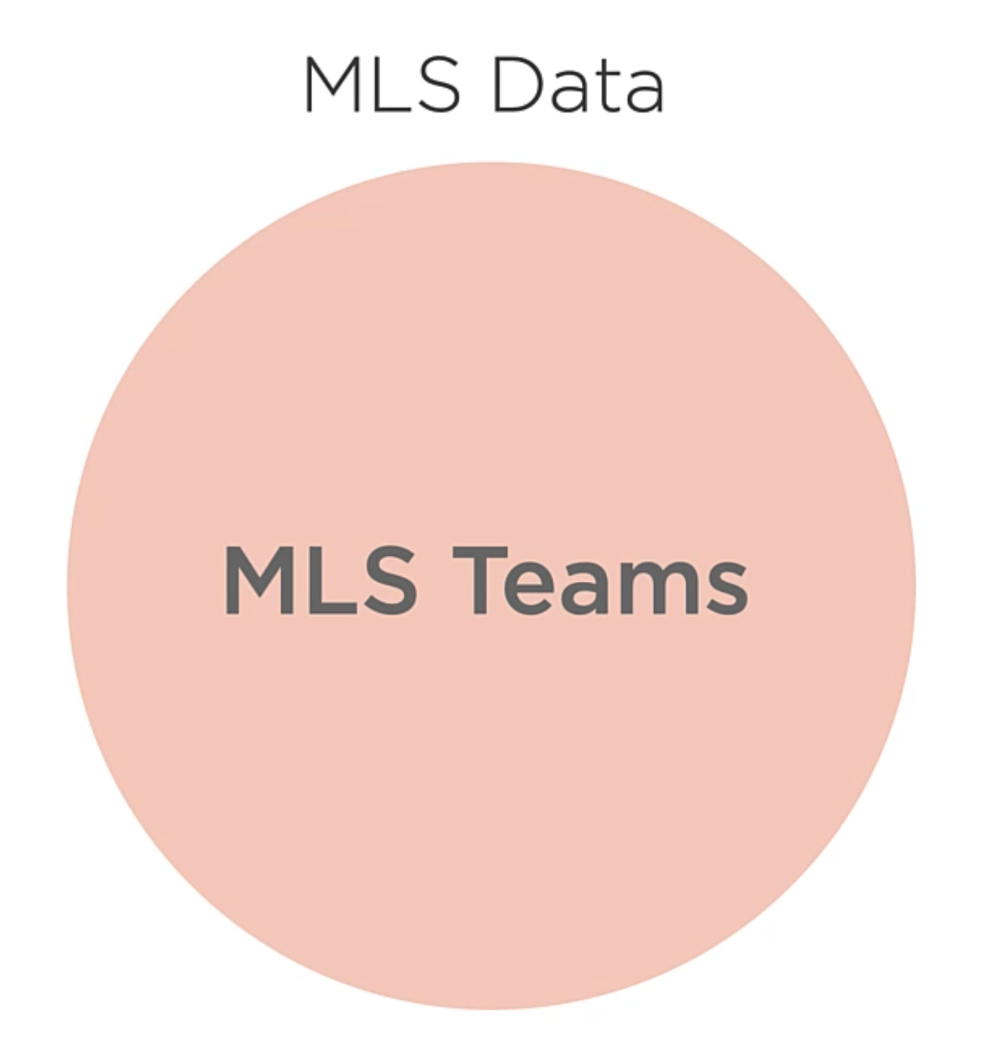
So, this circle represents a set of MLS, or Major League Soccer, teams. Through this module, we’ll use circles to represent sets and the data they contain. Let’s add some theams into the set.
1 | Set<Team> teams = new Set<Team>(); |
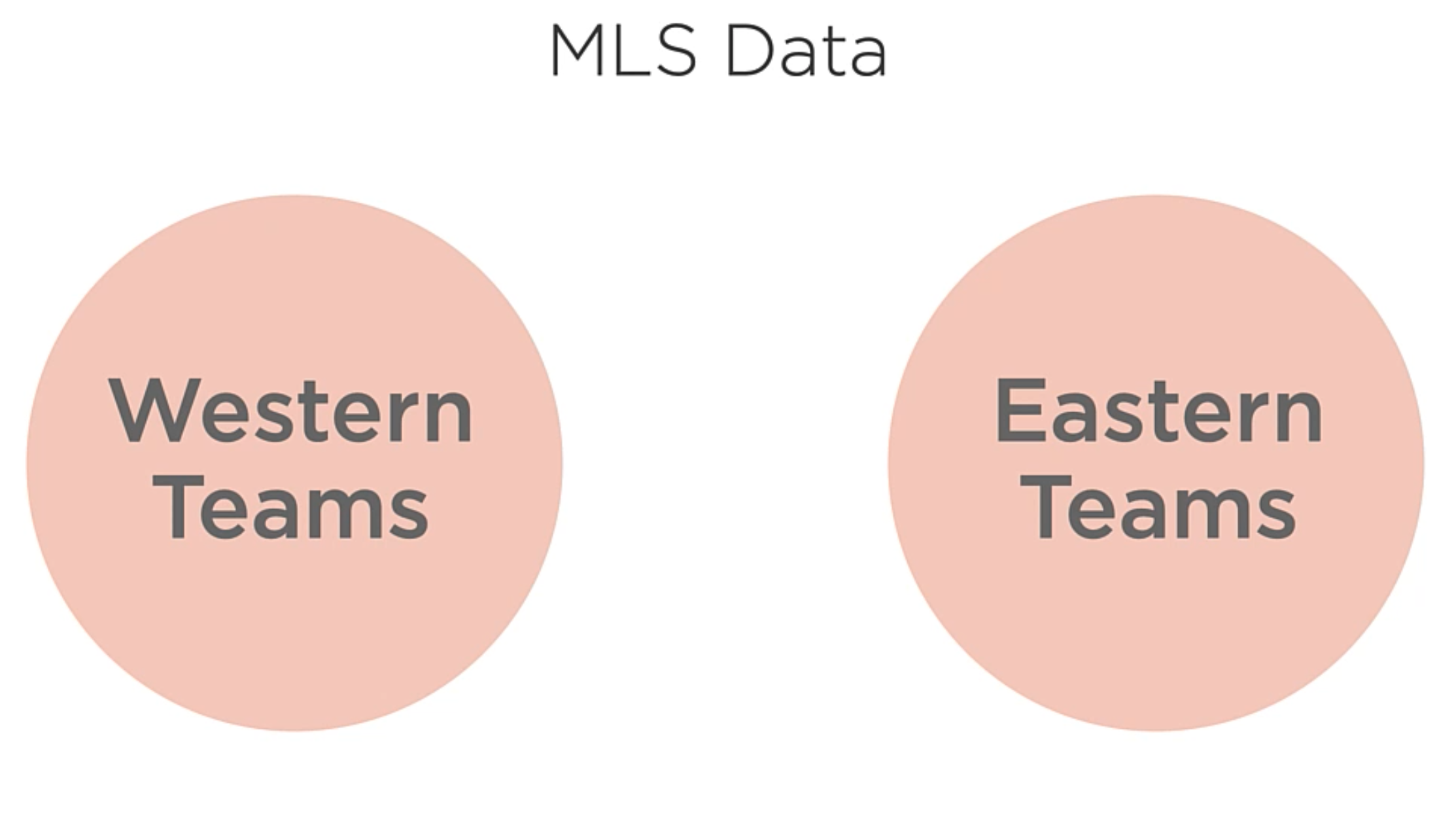
Another way to think of MLS teams is whether or not they’re in the Western or Eastern conference. So, each team is in one or the other, but not both.
1 | // Taking from the existing MLS teams Set and creating two new Sets |
It will looks like like this:
Set Operations: Union
The Set of all distinct items that exist within any of the input sets. This union operation of two sets produces a third set. This one will contain all of the distinct items in either of the input sets.
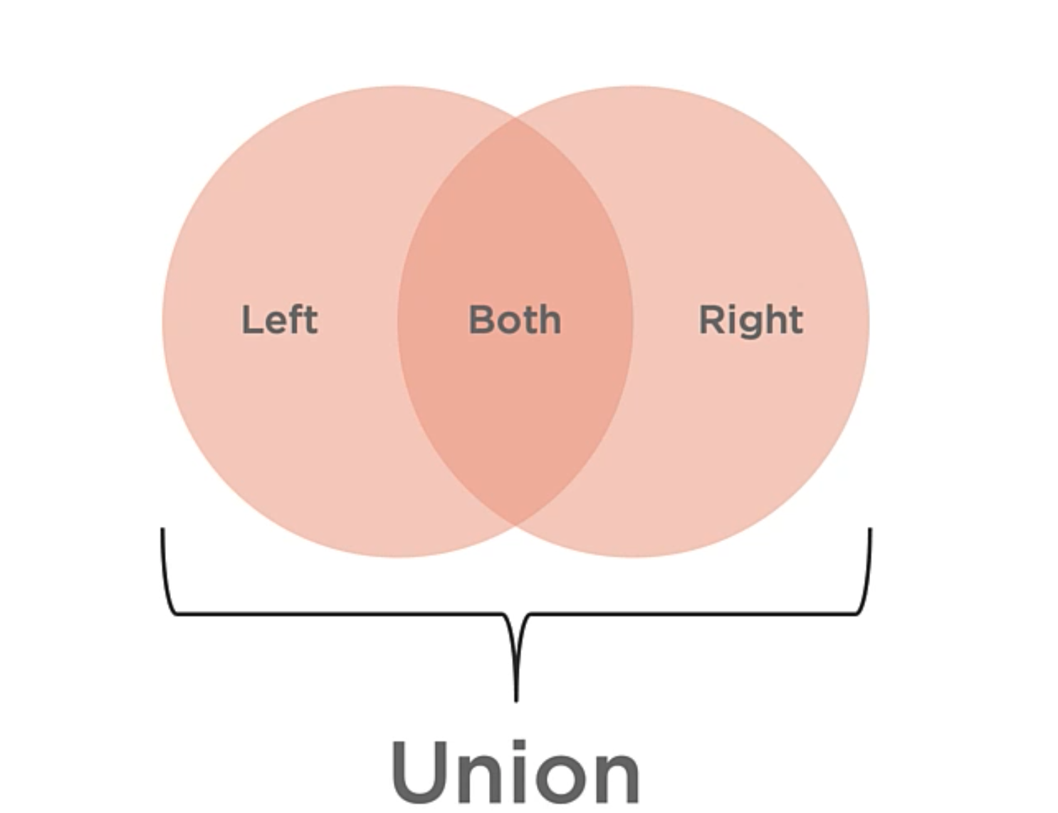
This operation can help to solve questions of “OR“. E.g. Which students are in Algebra or Biology?
A basic implementation of the union operation is shown below:
1 | ISet<T> Uion(ISet<T> other){ |
Set Operations: Intersection
The of items that exist within both input sets. The intersection of two sets creates a third set, which contains the items that exist within both input sets.
Let’s say we have two sets of students:
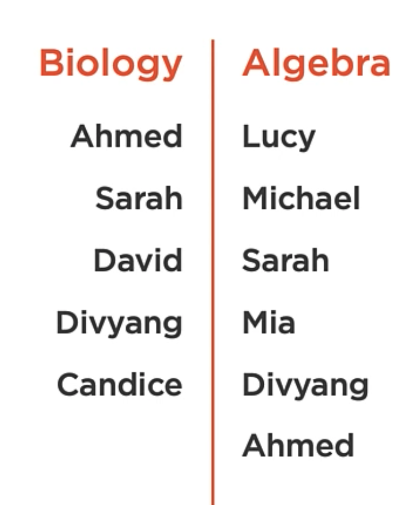
What if I wanted to know who is in both biology and algebra?
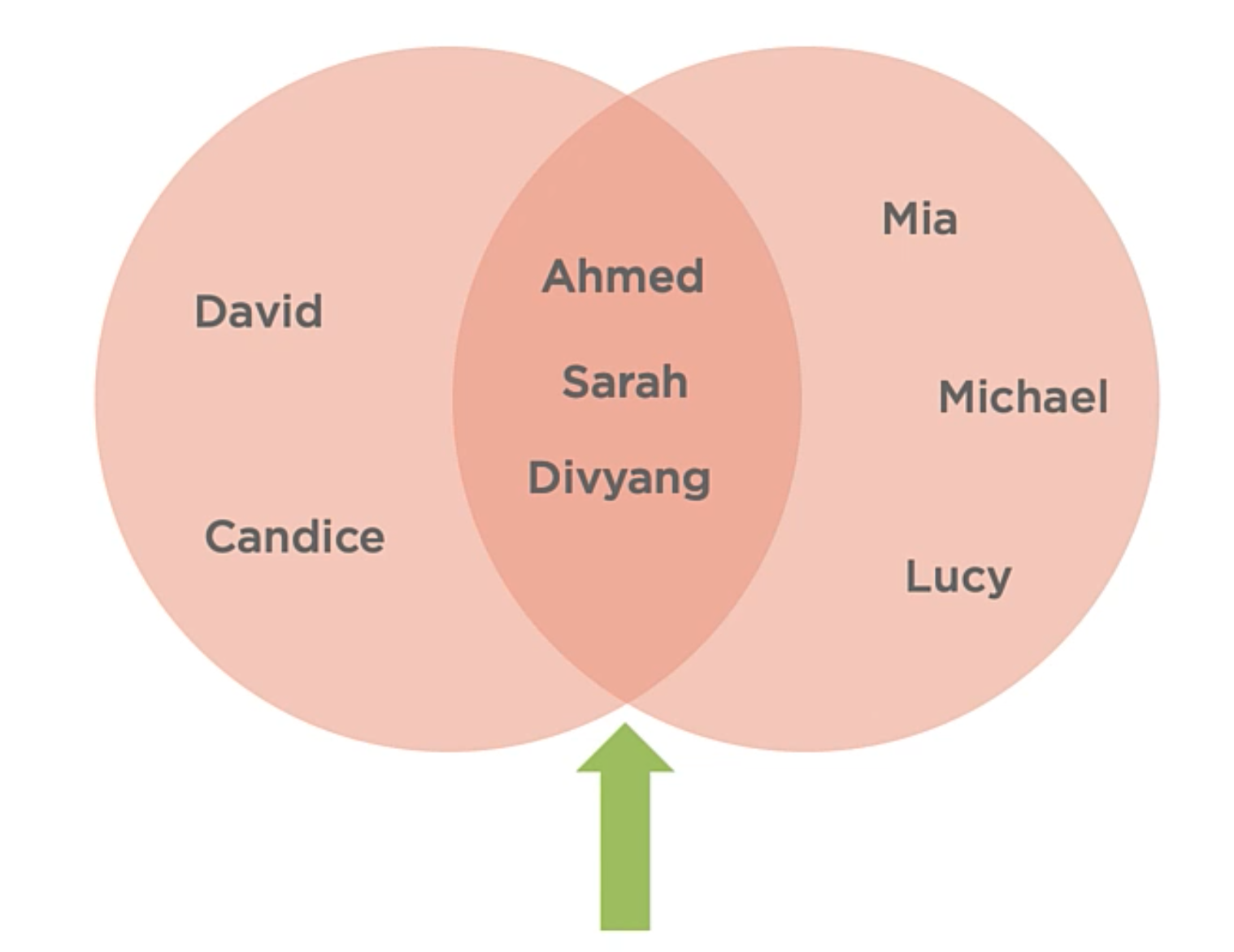
This operation can help to solve questions of “AND“. E.g. Which students are in Algebra and Biology?
A basic implementation of the intersection operation is shown below:
1 | ISet<T> Intersection(ISet<T> other){ |
Set Operations: Difference
The set of items which exist in one set which do not exist in the other.
Bringing back the example from above, we can ask the question, Which students are in Algebra but not in Biology?:
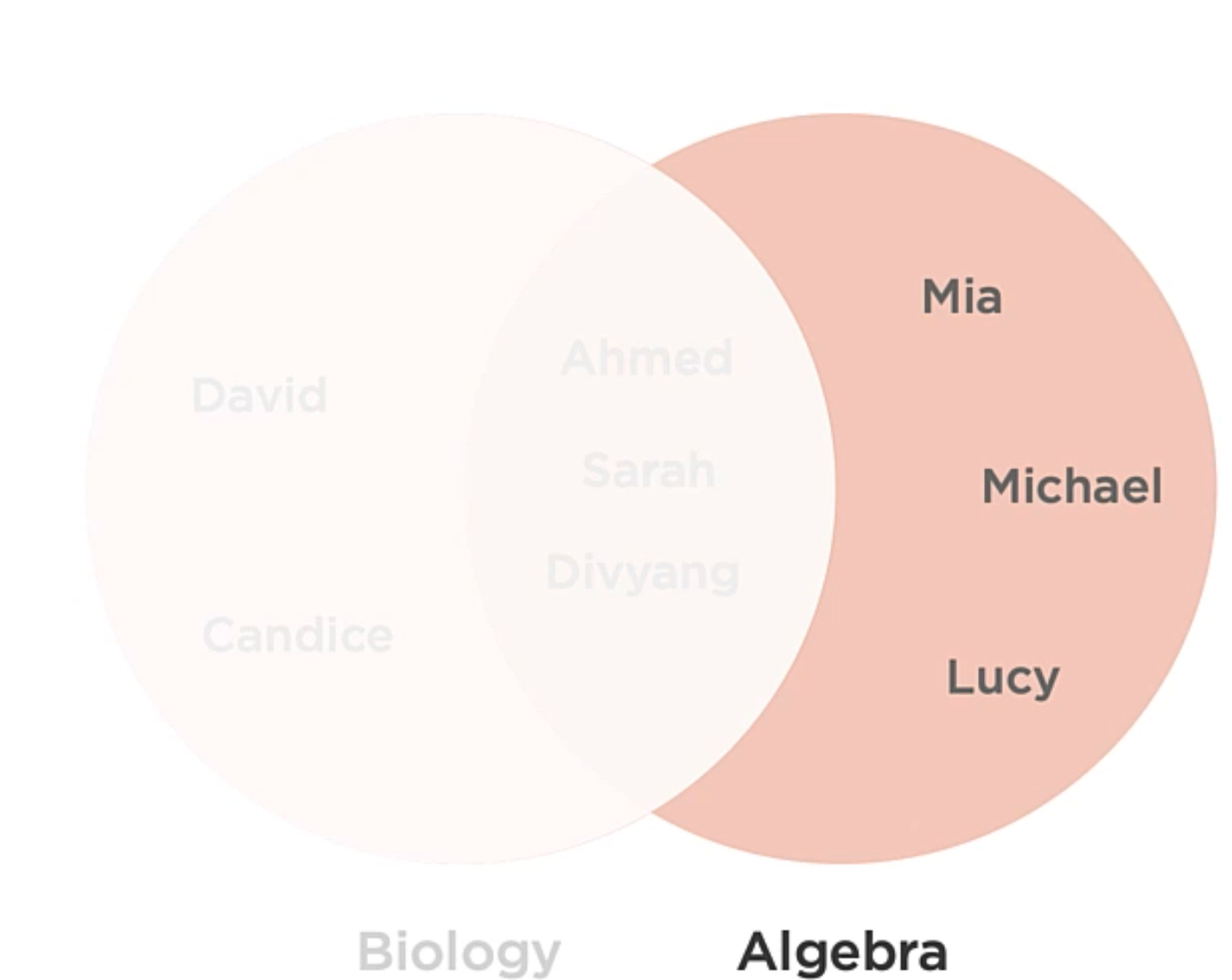
This operation can help to solve questions of “BUT NOT“.
A basic implementation of the difference operation is shown below:
1 | ISet<T> Difference(ISet<T> other){ |
Set Operations: Symmetric Difference
The set of items which exist in either of the two input sets, but which are not in ther intersection.
Bringing back the example from above, the symmetric difference would be something like this:
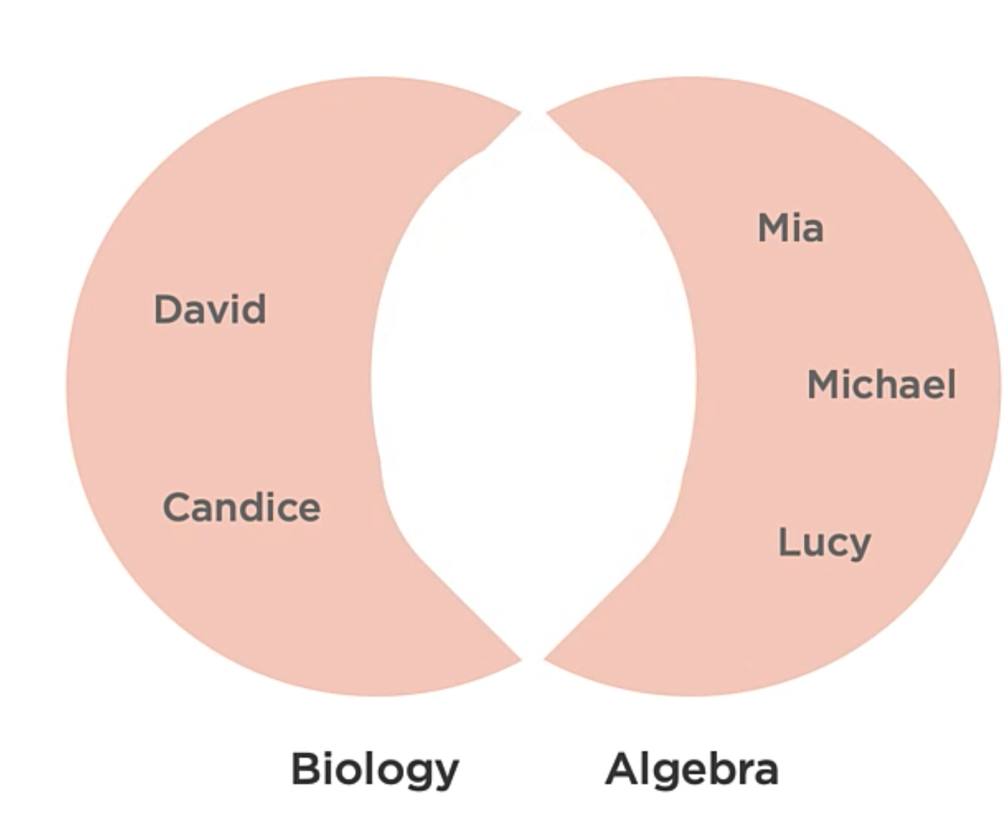
This operation can help to solve questions of “OR … BUT NOT BOTH“. E.g. Which students are in Algebra or Biology but not both?
A basic implementation of the difference operation is shown below:
1 | ISet<T> SymmetricDifference(ISet<T> other){ |
Code Example
With the set, you can get easyly the union, intersection, difference and symmetric difference of the sets.
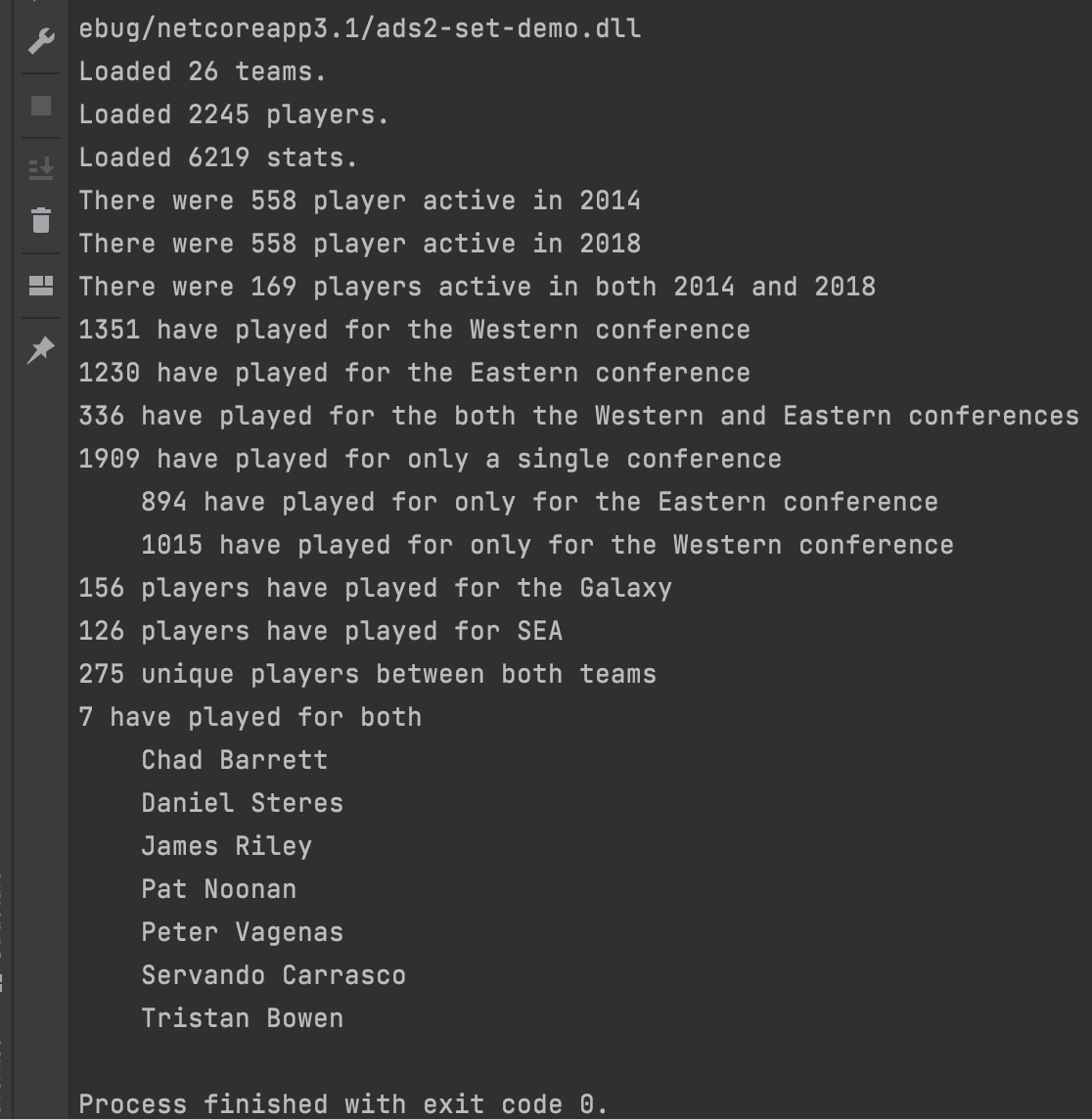
Here is the Set class implementation:
B-Trees
A b-tree is a sorted, balanced tree structure typically used to access data on slow mediums such as disk or tape drivers.
This is a b-tree.
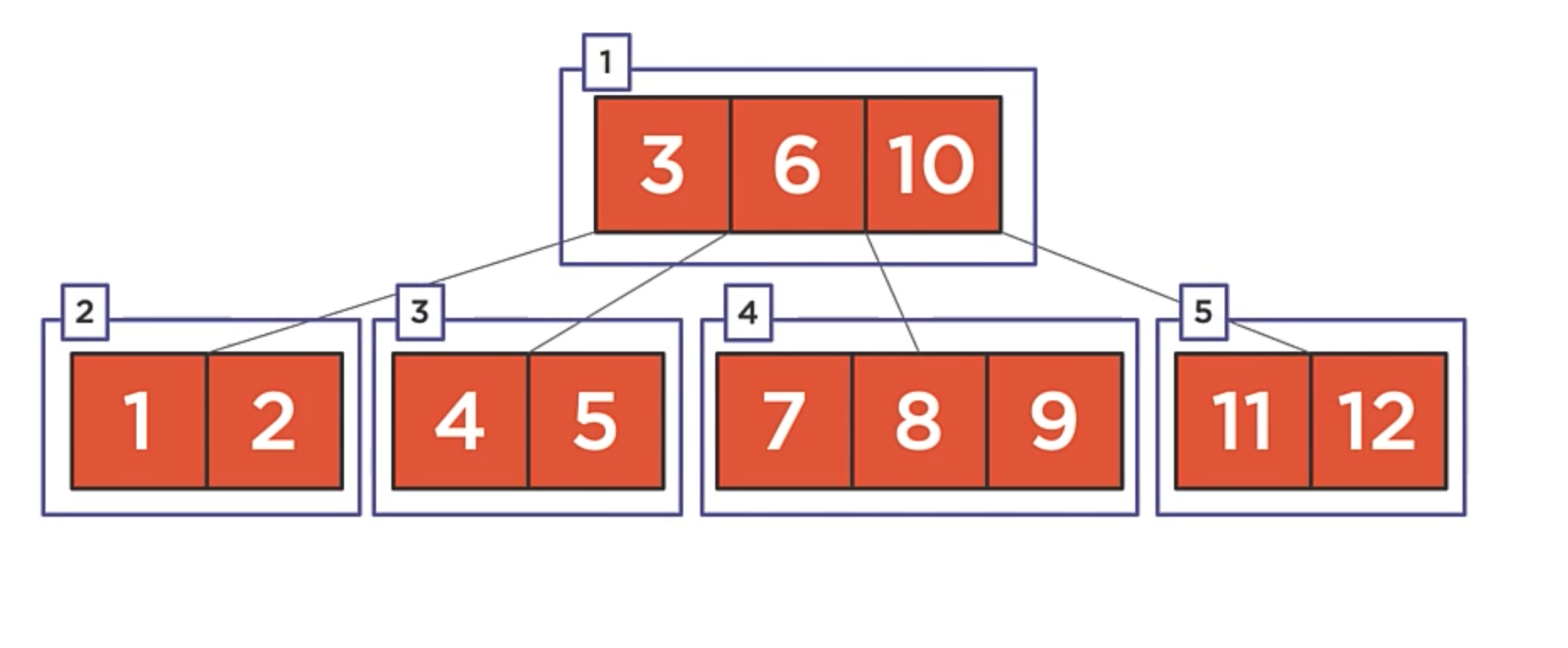
There is a couple of differences between a b-tree and the rest of the data structures we’ve seen so far.
- The root node contains the values [ 3 | 6 | 10 ]
- Binary trees have a single value per node, whereas b-trees can have multiple values per node.
- The root node has 4 children. Three of the children contain two values and one contains three values. That is also another difference with other binary trees. The b-tree have a maximum of two children per node.
- Notice that values in the b-tree are stored in a manner siminar to a binary search tree. Smaller values on the left and larger values on the right.
- This pattern of having one more child that it has values is an immutable property of the b-tree.
There is another example of a b-tree.
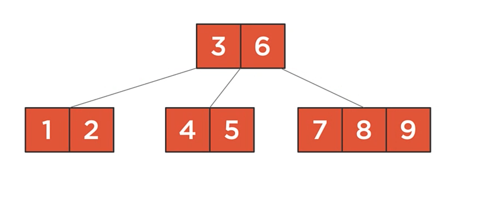
In this example:
- The root node has two values, so it has three children.

In this example:
- the root node has four values, so it has five children.
Nodes will always have one more child that values.
Add Rules
- Values can only be added to leaf nodes.
- Full nodes are split before the algorithm enters them (ensuring leaf nodes are never full before adding an item).

Splitting the root is the only way that the b-tree height increases.
Heaps and Priority Queues
Heaps
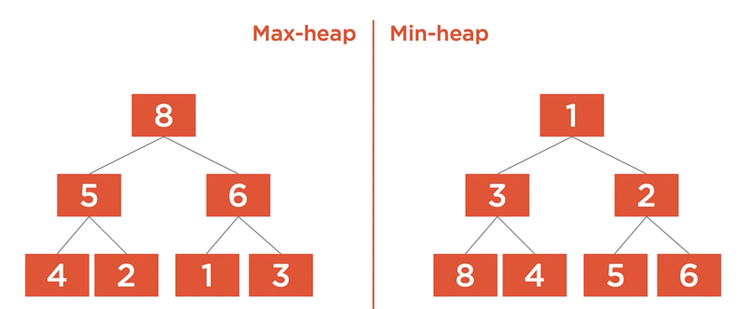
A heap is a tree-based container type that provides O(1) access to the minimim (min-heap) or maximim (max-heap) value while satisfying the heap property.
The heap property states that within the heap’s tree, every node’s value must be greater than or equal to all of its children’s values. This is true for the max-heap, but not for the min-heap. For a min-heap, the property is reversed. The value of the current tree item must be less than any of its child values.
Min-heap
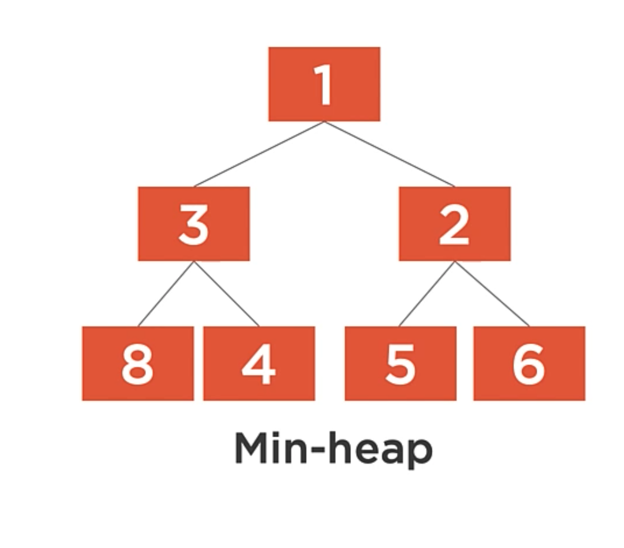
The min-heap must satisfy the heap property. For a min-heap, this means that for each node, its value must be less than or equal to all of its children’s values.
The implication of this is that the minimum value is always at the root of the tree. This is why we’re able to access the minimum value in O(1) time.
You can nitice that unlike a binary tree, there are no rules about the placement of the child values. The tree as shown is a valid heap, but we could move the 3,2 and 4 nodes around and still satisfy the heap property.
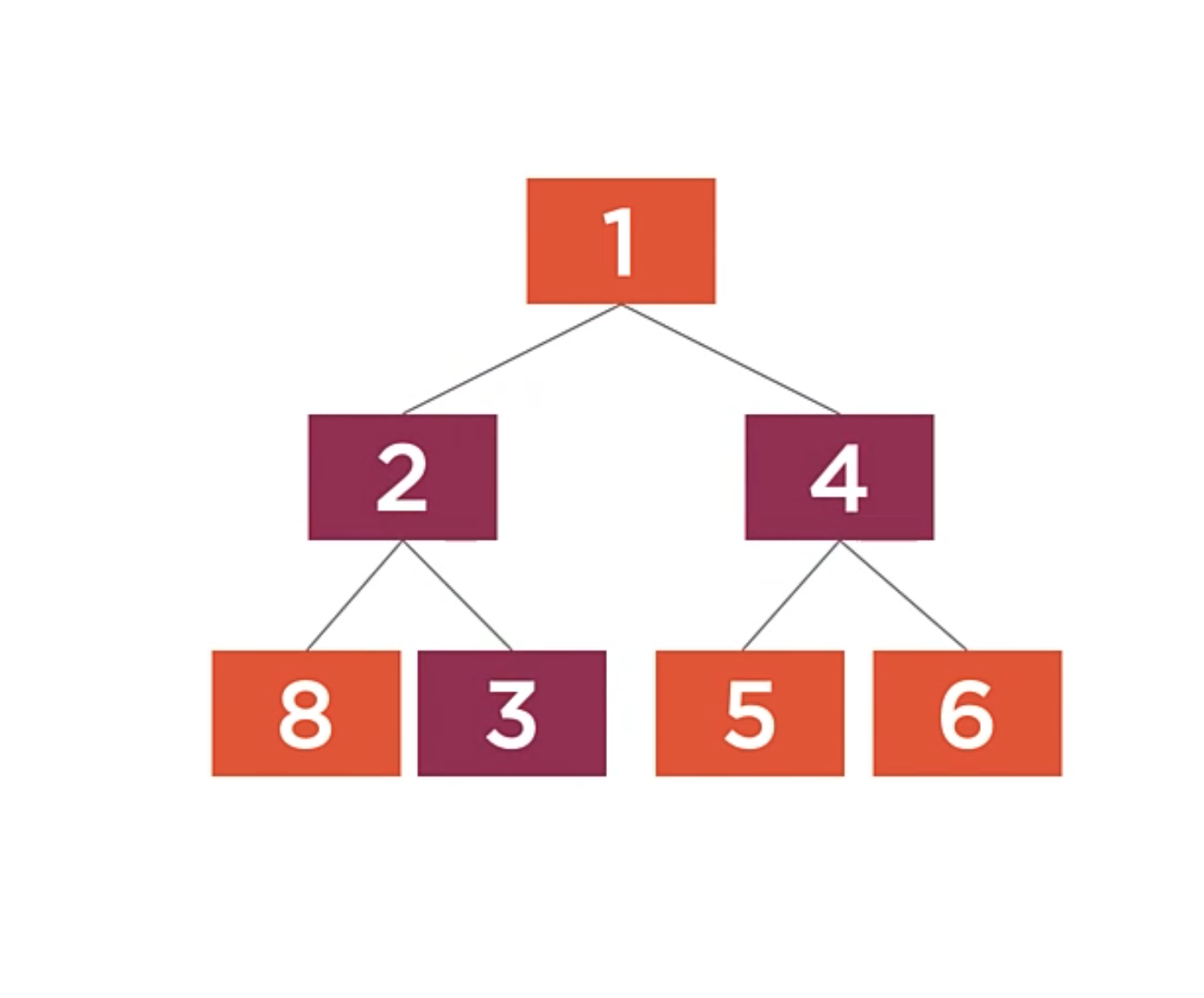
Max-heap
A max heap works the same way, only the heap property is reversed.

Collection Concurrency
Concurrency
Two or more operations executing at the same time (concurrently).
- Multiple threads executing within a single process accessing a shared resource (e.g. a shared List
) - Multiple processes running on the same computer accessing a shared resource (e.g. a shared file)
- Multiple processes running on different computers accessing a shared respource (e.g. a shared database table)
Resources
Understanding HashSet in C# with Examples | https://www.dotnetcurry.com/csharp/1362/hashset-csharp-with-examples
Using Advanced Data Structures in Modern Applications | https://app.pluralsight.com/library/courses/using-advanced-data-structures-modern-applications/table-of-contents
The Job Interview Guide 💼 | https://gist.github.com/jdnichollsc/b9bedff406b54c3ae2cd651512683b51